We encourage everyone to use the Wiradjuri names gifted to our Parkes Observatory telescopes. For example, the 64m telescope should be referred to as ‘Murriyang, CSIRO's Parkes radio telescope’ in the first instance in publications, presentations and general communication. Once the dual name has been used, the telescope(s) can be referred to more informally, for example as ‘Murriyang’, ‘the Parkes telescope’ or ‘The Dish’, at the discretion of the author or speaker. You may also wish to acknowledge the Wiradjuri people as the Traditional Owners of the Observatory site. Using the telescopes' Wiradjuri names acknowledges and respects the connection Wiradjuri People have to the land on which the telescopes sit.
This manual describes how to apply for observing time, make an observing schedule and carry out observations with Murriyang, the 64m CSIRO Parkes Radio Telescope. This manual is a reference and you should not feel that you must read all of it in order to use Murriyang. Chapter 1 describes the telescope system, including the characteristics of the available receivers and backends. This information can be used before proposing to use the telescope, the procedure for which is also detailed in this chapter. Chapter 2 can be read after being given observing time on Murriyang, as this chapter focuses on preparations needed to observe with Murriyang. Chapter 3 is dedicated to observing procedures and systems and details how to actually do your observations. Chapter 4 walks you through processes that occur once your observations are over, such as accessing your data and reporting your experiences.
In 2019 April there was a major overhaul of this manual: the presentation of the document on the web and in print was improved, and the content was significantly updated. Copies of this manual and other ATNF documentation can be obtained from the ATNF webpages.
If you find that any part of Murriyang doesn't work as described
in any of our documentation, please email the Murriyang Users Guide
editorial team at <ATNF-Parkes-Remobs[at]csiro.au>.
Comments on documentation are especially welcomed.
- 05th Nov 2025: Update 13mm conversion system scripts.
- 02nd Jul 2025: Added information on SSH access changes to ATNF machines venice and orion.
- 09th Apr 2025: Updated method to update PSRCAT on joffrey.
- 30th Jun 2024: Updated information on restarting CS-Studio on the joffrey VNC.
- 11th Mar 2024: Removed DFB4 (now retired), updated references to the new Observing Expert model and calendar implementation in PORTAL.
- 12th Feb 2024: Added gain-elevation curves for Mars and UWL receivers.
- 03rd Nov 2022: Removed Galileo, SX and AT-Prototype as offered receivers.
- 13th Oct 2022: Updated Mars configuration on Medusa to an LO setting of 8457 MHz; was 8500 MHz.
- 10th Jun 2022: Added SPOT continuum mode for pointing purposes.
- 16th May 2022: Remove TOS import, added information on observing with MARS/13MM receivers.
- 20th Apr 2022: Added information on setting up MARS/13MM receivers and Dhagu? integration.
- 17th Mar 2022: Added information on the NoDrive observing mode.
- 07th Mar 2022: Added info on Observing Queue being disabled if wind parked.
- 27th Aug 2021: Added gain-el curves for UWL at 1.38, 3.1 and 3.3 GHz
- 29th Jul 2021: Added 13mm gain-el curve at 23916 MHz.
- 13th Jul 2021: Added 13MM gain-el curve at 22387 MHz.
- 28th Jun 2021: Removed 0407-658 as a continuum calibrator as there is no well-defined flux model. Use 0823-500 or 1934-638 for frequencies less than 10 GHz.
- 15th Jun 2021: It is no longer possible to select the mode of a scan as small or great-circle. This is done internally, with the condition lat1==lat2 for the endpoints results in a small-circle scan, great otherwise. The joffrey command "makePSRCAT_backends" now pushes the current version of PSRCAT to Dhagu?, but note a logout/login of Dhagu? is required to pick up the changes.
- 31st May 2021: 'field_comment' in a CSV import file is now 'comment'. Removed option to select small/great circle scans.
- 26th May 2021: Updated 13MM Tsys/Tcal plots.
- 18th May 2021: Improved Moon Tsys/Tcal plots for some receivers. Removed H-OH receiver (superceeded by UWL.)
- 4th Apr 2021: Updated text and figures associated with scanning modes as the scan type can now be defined as a small or great-circle scan.
- 11th Mar 2021: Clarified definition of the output_tsubint parameter.
- 1st March 2021: Lowered supported Firefox on Debian to v78.
- 19th Feb 2021: Added field_comment to CSV import in Dhagu?
- 28th Oct 2020: Added information on supported web browsers.
- 23rd Sep 2020: Included Tsys/Tcal plots for the 13MM receiver. Updated information on Dhagu? release v0.10.0 .
- 20th Jun 2020: Updated information on accessing Medusa from outside the ATNF/CSIRO network.
- 1st May 2020: Updated Medusa search mode coherent dedispersion and DM parameters. These were based on a subband level, but are now configurable at the target (source) level.
- 21st Apr 2020: Updated Dhagu? screenshots to tie in with removal of AzEl offsets. Added Scan, ScanMap examples. Medusa tab in Dhagu? explained, and update on Medusa commensal modes. Added in receiver characterization.
- 6th Apr 2020: Addition of commensal observing modes in Dhagu?
- 9th Mar 2020: Updated Dhagu? descriptions, including new ScanMap implementation.
- 22nd Nov 2019: Transfered over to Docbook format.
In this manual we use some typographical conventions to help clarify the documentation.
Computer system names, e.g. joffrey
Software packages, e.g. psrcat
Software program, e.g.
pdfb4
Command example, e.g. $ df -h
Filename, or file content, e.g.
output.txtProgram option, e.g.
enable tsysSingle parameter name, e.g.
common.targetsAstronomy-related acronym, e.g. USB (upper sideband)
Non-astronomy-related acronym, e.g. USB (universal serial bus)
Table of Contents
- Preface
- 1. Murriyang, the CSIRO Parkes Radio Telescope
- 2. Preparing your observations
- 2.1. Calibration
- 2.2. Injected Calibration
- 2.3. Calibration Sources
- 2.4. Creating Parameter Sets
- 2.5. Viewing and Saving the Parameter Set
- 2.6. Loading Saved Parameter Sets
- 2.7. Example Pulsar FOLD Parameter Set
- 2.8. Example Pulsar SEARCH Parameter Set
- 2.9. Example CONTINUUM (Spectral-line) Parmameter Set
- 2.10. Example SCANMAP CONTINUUM (Spectral-line) Parmameter Set
- 2.11. Example SCAN Parmameter Set
- 2.12. Example FOLD Parameter Set: J0835-4510 with MARS
- 3. Observing with Murriyang
- 4. After your observations
- Index
The Australia Telescope National Facility (ATNF) is managed as a National Facility by the Commonwealth Scientific and Industrial Research Organisation (CSIRO). Formerly part of the CSIRO Division of Radiophysics, it became a separate division in January 1989. The ATNF became a National Facility in April 1990. In December 2009, ATNF became part of a new Division, CSIRO Astronomy and Space Science (CASS), together with NASA Operations (including the Canberra Deep Space Communication Complex), and CSIRO Space Sciences and Technology. The Australia Telescope continues as a National Facility, providing world-class observing facilities for astronomers at Australian and overseas institutions.
The majority of ATNF staff are located at the headquarters in Marsfield, a suburb of Sydney in New South Wales – although Marsfield is sometimes referred to as ‘Epping’, a larger, neighbouring suburb. A growing number of ATNF staff are also located in the Perth suburb of Kensington, Western Australia at the Australian Resources Research Centre (ARRC).
Besides Murriyang, the ATNF operates the Australia Telescope Compact Array (ATCA) which is comprised of an array of six, 22-m antennas and is located in Narrabri, NSW. ATNF also is currently commissioning the Australian Square Kilometre Array Pathfinder (ASKAP). The telescope has been constructed by ATNF in Murchison, Western Australia, and is an array of thirty-six wide-field 12m antennas operating in the 0.7–1.8 GHz range. More details are available on the ASKAP project website. Additionally, the ATNF negotiates time with the CSIRO-administered 70-m and 34-m antennas at the Tidbinbilla Deep Space Tracking station outside Canberra. The ATNF telescopes are used together, in conjunction with the University of Tasmania telescopes at Hobart and Ceduna, as part of the Long Baseline Array for Very Long Baseline Interferometry (VLBI) observations.
The Parkes Observatory is located 415 m above sea level at Latitude -32.99839 South, Longitude 148.26352 East, 25 kilometres north of the town of Parkes which is approximately 365 kilometres west of Sydney. It is 6 kilometres off the Newell Highway, the main road from Parkes to Dubbo. The Shire has a population of 15,000 and the town a population of 10,000 and is in the middle of a rich sheep, wheat producing and mining area. Table 1.1 gives an accurate site location in Cartesian coordinates and Table 1.2 lists Murriyang's geodetic coordinates in both WGS84 and AGD84/AHD systems. The Murriyang position was derived from VLBI measurements on 2016-December-19. See the ATNF online appendix for more information on observatory coordinates and calculations.
Figure 1.1 shows a complete site overview of the Parkes Observatory. The site contains Murriyang, the 64-metre Radio Telescope, Giyalung Miil, the 12-metre ASKAP prototype antenna, the now decommisioned 18-meter Giyalung Guluman, or "Kennedy Dish", an administration building with offices, workshops and library, Visitors Discovery Centre and The Dish Cafe. In addition, there are numerous testing and monitoring facilities on site.
Table 1.1. Location of Murriyang in Cartesian coordinates.
| X(m) | e(X) (m/yr) | e(Y) (m/yr) | e(Y) | Z(m) | e(Z) (m/yr) |
|---|---|---|---|---|---|
| -4554231.5380 | -0.03425 | 2816758.8656 | -0.00301 | -3454034.9686 | 0.04837 |
Table 1.2. Geodetic coordinates of Murriyang.
| Coordinate System | Longitude (deg) | Latitude (deg) | Longitude (DMS) | Latitude (DMS) | Spheroidal (m) |
|---|---|---|---|---|---|
| WGS84 | 148.2635101 | -32.9984064 | 148 15 48.636 | -32 59 54.263 | 410.80 m |
| AGD84 | 148.2623007 | -32.9999629 | 391.52 m | 148 15 44.283 | -32 59 59.866 |
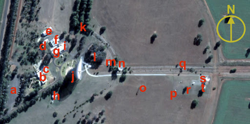
Overview of the CSIRO Parkes Radio Observatory. The letters correspond to the following locations on site: a) Visitor car park b) Visitor Centre c) `The Dish’ cafe d) carpenter workshop e) welding hut and equipment shed f) mechanical and electrical workshop g) admin building (“Opera House”) h) generator hut i) receiver lab j) the tower k) staff and service road l) staff tea area and RFI lab (“the woolshed”) m) maser hut n) mobile interferometer (“kennedy antenna”) o) wind station and RFI reference (“Telstra tower”) p) 3.7m antenna q) RFI monitoring tower r) hot/cold testing s) 12m antenna (“ASKAP antenna”) t) Harold’s hut.
The observatory can be contacted at the following address:
        CSIRO Parkes Observatory
        473 Telescope Road (or PO BOX 276)
        PARKES NSW 2870
        Australia
        Switch:(02) 6861 1700 [International +61 2 6861 1700]
        Fax: (02) 6861 1730 [International +61 2 6861 1730]
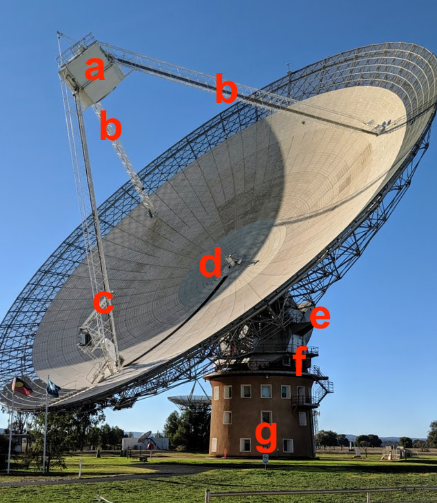
Figure 1.2. Overview of the tower. The letters correspond to the following: a) aerial/focus cabin b) feed legs c) lift leg d) vertex radiator e) counterweight f) azimuth track g) control tower.
The antenna has a paraboloid design with a 64-m diameter. The surface is high precision aluminium millimetre wavepanels to a diameter of 17-m (for operation to 43 GHz), then perforated aluminium plate out to 45-m, and rectangular galvanised steel 5/16-inch mesh for the remainder of the surface. The focal ratio is 0.41 for the full 64m surface, the focus being located 26-m above the centre.
The aerial cabin, which houses feeds and receiver equipment, is supported by a tripod. Access to the aerial cabin is either by the lift on one of the tripod legs (the “lift leg”) or by a ladder on one of the other legs. The feed platform translator, which can hold up to four receivers, at the base of the aerial cabin has up/down (focus), lateral and rotational movement. Figure 1.2 labels these and other commonly referenced parts of the telescope.
Further properties of the Radio Telescope are shown below.
        Weight of counterweight: 475 tonnes
        Total weight of dish: 1,000 tonnes
        Surface area of reflecting mesh: 0.4 hectares (1 acre)
        Height of concrete tower: 10.7 m (35 ft)
        Height to centre of dish: 27.4 m (90 ft)
        Height to top of aerial cabin: 58.6 m (192 ft)
        Power of azimuth/zenith drives: 11kW (15 hp)
        Pointing accuracy:  < arcsec
        Sky coverage:
        Az: 0-360 deg.
        El: 30.5 - 88.5 deg.
The dish may be operated between the Zenith angle software limits of 1.2 and 59.5 degrees. There are three hardware limits at Zenith angles less than 1.5 degrees, and also another three past 59.5 degrees. The dish can be “stowed” at a physical limit 30 minutes of arc beyond the Zenith. It is constrained in this position by a locking pin. Azimuth angle is measured as 0 degrees due north, increasing to the east.
The Ultra Wide-bandwidth Low (UWL) receiver system provides continuous frequency coverage from 704 - 4032 MHz. The feedhorn design is described in detail in Dunning et al. (2015), and the feed achieves a near constant beam width over a 6:1 bandwidth (note that the beam on the sky still scales with λ/D). Over the majority of the band, there is a system temperature of ~20 K and the system remains linear even in the presence of strong RFI.
For the first time, the band is digitised in the focus cabin into three distinct bands (`low’, `mid’ and `high’). Each band is then passed to field programmable gate arrays (FPGAs) which are used to receive the digitised signal and produce a total of 26, 128 MHz subbands. The frequency range and corresponding sub-band number are given in Table 1.3 As of September 2019, the UWL filterbank is critically sampled, introducing roll-off at the edges of each sub-band. This will restrict the ability to study spectral lines +/- 5 MHz from the sub-band edges. This does not discount these frequencies, but observations will suffer lower than average sensitivity and there is the potential for aliasing if a source is particularly bright.
Table 1.3. Frequency coverage for each of the 26, 128-MHz sub-bands as processed by the FPGAs and referenced by the MEDUSA backend. The table also shows the breakdown into the three distinct digitised bands: low, mid and high.
| Low Band | Mid Band | High Band | |||
|---|---|---|---|---|---|
| Frequency Range (MHz) | Sub-band number | Frequency Range (MHz) | Sub-band number | Frequency Range (MHz) | Sub-band number |
| 704-832 | 0 | 1334-1472 | 5 | 2368-2496 | 13 |
| 832-960 | 1 | 1472-1600 | 6 | 2496-2624 | 14 |
| 960-1088 | 2 | 1600-1728 | 7 | 2624-2752 | 14 |
| 1088-1216 | 3 | 1728-1856 | 8 | 2752-2880 | 16 |
| 1216-1344 | 4 | 1856-1984 | 9 | 1880-3008 | 17 |
| 1984-2112 | 10 | 3008-3136 | 19 | ||
| 2112-2240 | 11 | 3136-3264 | 19 | ||
| 2240-2368 | 12 | 3264-3392 | 20 | ||
| 3392-3520 | 21 | ||||
| 3520-3648 | 22 | ||||
| 3648-3776 | 23 | ||||
| 3776-3904 | 24 | ||||
| 3904-4032 | 25 | ||||
Once the data has been packetised in the FPGAs, it is sent to the GPU correlator (or backend) called “MEDUSA”. Note we use APOLLO processing threads on MEDUSA for Fold, Search and Continuum modes with the UWL and legacy receiver observing (MARS, 13MM), and BOREAS threads for the CRYOPAF Timing, Search and Galactic (Continuum) modes.
Table 1.5. Normalized gain-elevation curves of the form:
| A0 | A1 | A2 | A3 | Freq/BW (MHz) | Date |
|---|---|---|---|---|---|
| 0.846669 | 0.574301E-02 | -0.575373E-04 | 0 | 3200/128 | Mar 2023 |
| 0.943957 | 0.128698E-02 | -0.974358E-05 | 0 | 1408/128 | Mar 2023 |
| 0.757765 | 0.816472E-02 | -0.687898E-04 | 0 | 1380/64 | Jul 2020 |
| 0.635072 | 0.128570E-01 | -0.1113244E-03 | 0 | 3100/64 | Apr 2020 |
| 0.624774 | 0.766677E-02 | -0.391624E-04 | 0 | 3100/64 | Nov 2018 |
| 0.803516 | 0.739070E-02 | -0.695002E-04 | 0 | 3300/64 | Sept 2021 |
For a complete description of the system installed on Murriyang, as well as a summary of system temperature, beam efficiencies/FWHM and RFI across the observing band, see Hobbs et al. (2019).
This is a dual package, with the upper frequncy range 12.0 - 12.8 GHz, and the lower 5.9 - 7.0 GHz. However, the upper frequency range is not operational. For the lower range, one of either of the LNAs is known to oscillate from time to time, but never both. This tends to settle down after the LNAs have been left on for some time.
Table 1.7. Normalized gain-elevation curves of the form:
| A0 | A1 | A2 | A3 | Freq/BW (MHz) | Date |
|---|---|---|---|---|---|
| 0.595086 | 0.138104E-01 | -0.117758-03 | 0 | 6666/1024 | Mar 2020 |
| 0.562466 | 0.144946E-01 | -0.123892E-03 | 0 | 6666/64 | Oct 2013 |
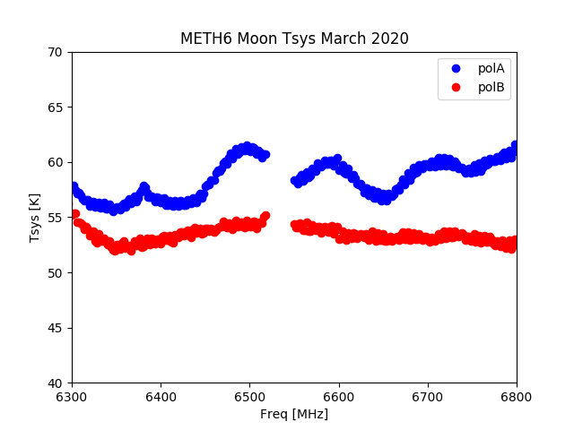
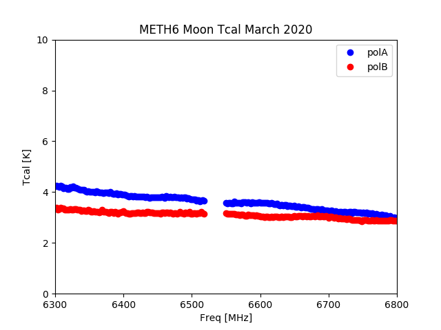
The following plots show the system and calibration temperature of the METH6 receiver (Kelvin). The Moon was used for the measurements, with correction for opacity, plus contributions from atmosphere and ground emission included.
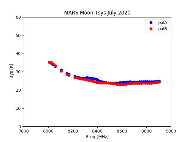
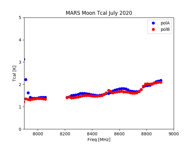
A receiver built to track NASA mars missions. The MARS (8.4 GHz; X–band) receiver has a built-in (non-removable) waveguide circular polariser also with cal injection between the polariser and OMT.
Table 1.9. Normalized gain-elevation curves of the form:
| A0 | A1 | A2 | A3 | Freq/BW (MHz) | Date |
|---|---|---|---|---|---|
| 0.271 | 0.364E-01 | -0.343E-03 | 0 | 8457/128 | Aug 2025 |
| 0.132609 | 0.321718E-01 | -0.304819E-03 | 0 | 8329/128 | Sep 2023 |
| 0.158093 | 0.325514E-01 | -0.316076E-03 | 0 | 8329/128 | May 2023 |
| 0.13932 | 0.333776E-01 | -0.323993E-03 | 0 | 8329/128 | Dec 2022 |
| 0.420982 | 0.212328E-01 | -0.194654E-03 | 0 | 8400/1024 | Mar 2020 |
| 0.369170 | 0.249620E-01 | -0.230021E-03 | 0 | 8425/64? | Mar 2015 |
| 0.675138 | 0.127966E-01 | -0.126014E-03 | 0 | 8425/64? | Aug 2013 |
| 0.790027 | 0.336820E-02 | 0.850692E-04 | -0.139814E-05 | 8425/64? | Aug 2003 |
The following plots show the system and calibration temperature of the MARS receiver (Kelvin). The Moon was used for the measurements, with correction for opacity, plus contributions from atmosphere and ground emission included.
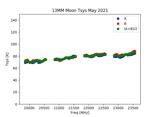
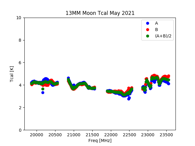
A K-band receiver covering 16-26 GHz was delivered and commissioned in September 2008 and July 2009. The receiver has wider frequency coverage than the older K-band receiver and appears to have the anticipated ~threefold advantage in Tsys at 22 GHz over the older package. The receiver can be installed with either of two feeds: a narrow- band feed and quarter-wave plate providing dual orthogonal circular polarisation over the frequency range 21.0 to 22.3GHz, or the standard feed providing dual orthogonal linear polarization over the 16 to 26GHz range. The package has two independent conversion systems allowing simultaneous operation at any two arbitrarily-spaced frequencies within the band limits. The 13MM receiver also has an optional quarter-wave plate used with the narrow-band VLBI feed covering the 22 GHz water transition. The cal injection occurs after the polariser (between the polariser and the OMT). More information on the receiver is available here.
Table 1.11. Normalized gain-elevation curves of the form:
| A0 | A1 | A2 | A3 | Freq/BW (MHz) | Date |
|---|---|---|---|---|---|
| -0.315708 | 0.734205E-01 | -0.126417E-02 | 0.625803E-05 | 23916/900 | July 2021; tau_0 = 0.03 +/- 0.01 neper |
| -0.617938 | 0.631747E-01 | -0.616688E-03 | 0 | 22387/900 | July 2021; tau_0 = 0.06 +/- 0.01 neper |
| 0.945760 | 0.373780E-01 | -0.385728E-03 | 0 | 22236/64? | Sept 2012 |
The following plots show the system and calibration temperature of the 13MM receiver (Kelvin). The Moon was used for the measurements, with correction for opacity, plus contributions from atmosphere and ground emission included.
The overall outline of the observing system is shown in Figure 1.9.
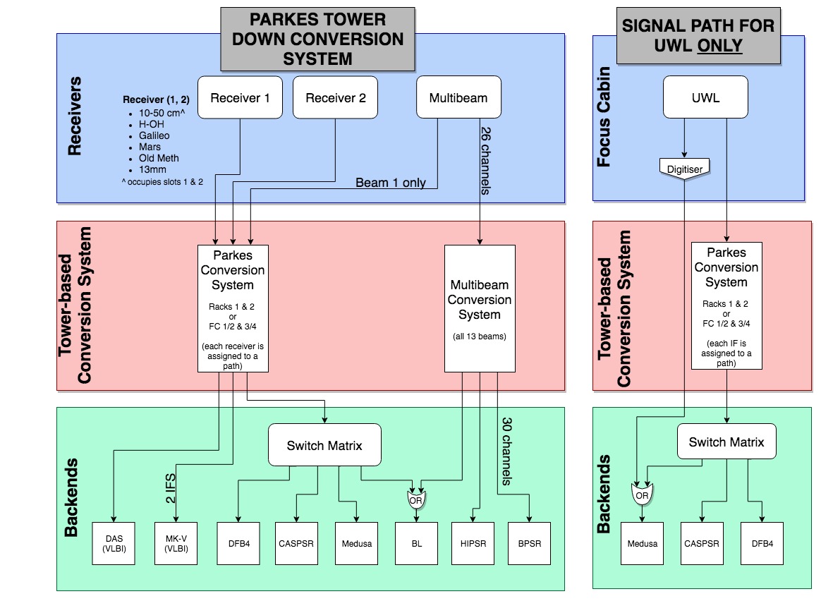
Since February 2019, MEDUSA has become the dominant backend for all observations with the UWL. In the normal operation of the UWL in conjunction with MEDUSA, the full UWL band is digitised into three discrete bands in the focus cabin. Each of these bands is sent down to the control tower to a suite of FPGAs, where the data are broken into further sets of 128 MHz sub-bands. Data are then sent to the MEDUSA GPU cluster where it is processed according to the user-defined observing parameters (See Section 1.3 Observing Modes for full details on the capabilities of each mode).
The legacy Conversion System (PCS) has been the main method of down-conversion for all single-pixel feed receivers. However, the introduction of the UWL and the tower digitisers means receivers other than the UWL still use the PCS for feed-through to Medusa, or other thried-party backends. An in-depth discussion of the PCS is available here (PDF file).
When preparing your observing proposal, you are required to estimate the expected brightness and sensitivity of your source for your particular correlator/receiver combinations. For spectral-line observations, sensitivity per bandwidth channel can be estimated from the following equations of line brightness and line flux respectively:
In the above, G is the main-beam gain (Jy/K) for a receiver defined from where and are the solid angles on the sky for the main beam and the total collecting are of the antenna, respectively. Also, npol is the number of polarisations (an average of two independent polarisation channels), BW is the bandwidth [MHz], nchan is the number of channels and is the on-source integration time in seconds. is the beam efficiency factor = 0.7. For continuum, we need to calculate the sensitivity over the whole bandwidth. The continuum line brightness and line flux respectively become:
For both the line and continuum flux, the source is assumed to fill the main beam which has efficiency G~0.7. The theoretical RMS noise estimates for line and continuum observations can be estimated using the on-line sensitivity calculator. A detailed analysis of the sensitivity calculator, with examples of data, is given here.
MEDUSA a GPU-based signal processing unit that was specifically designed to support the UWL receiver. Integration with other receivers is possible, though users are strongly encouraged to collaborate with local support to discuss and facilitate any such use cases.
MEDUSA is capable of processing each of the 26, 128-MHz sub-bands of the whole UWL bandpass independently. The processing can involve forming full polarisation products, folding these signals in a mode typical of “fold mode” pulsar observations, creating products suitable for searching for transient events (akin to “pulsar search mode”), and/or producing high-frequency resolution data for use in spectral line or continuum emission studies.
Each of the 26 sub-bands can be configured independently in any of the observing modes (search, fold, continuum, etc). See Section 1.3 for a summary of each mode or Hobbs et al. (2019) for a complete summary of the backend modes.
The suite of backend instruments available ensures that a diverse range of observations can be carried out. These are usually split into high time-resolution modes (e.g., pulsar observations) and high spectral-resolution modes (e.g., spectral line observations). In this section we describe the observing modes available for use with the Ultra-Wide-Low (UWL) receiver. The astronomy processing is initially carried out on a GPU cluster (known as “MEDUSA”) with subsequent processing on a CPU server (known as euryale).
If the pulsar astrometric, spin, dispersion measure and orbital parameters are known (from, e.g., a tempo2 timing solution) then the incoming data stream can be “folded” at the topocentric period of the pulsar. For each 128 MHz-wide sub-band, the data is coherently dedispersed and channelised. The data are then detected, polarisation products AA, BB, Real(A*B), Imag(A*B) formed and folded into pulsar phase bins. The data are output for every sub-integration. The data are output in a PSRFITS fold-mode data file. The switched calibration signal is not run during such observations; typically the calibration signal is recorded (using the same observing mode) prior to the pulsar observation.
User options:
Number of frequency channels/sub-band: between 64 and 4096 channels.
Number of pulsar phase bins: between 8 and 4096 bins
Sub-integration time: between 8 and 60 seconds
If a new pulsar is to be added to the folding catalogue, or the parameters for a particular pulsar requires updating then the following procedure should be followed (note that this will be simplified in the near future):
Log on to joffrey as pksobs (password required)
cd $PSRCAT_RUNDIR
Create a new obs*.db file (or update an existing one for your project). Note that formatting required (this is not exactly the same format that gets output as a TEMPO2 parameter file).
Test that the parameters are correct for your updated or new pulsar using: psrcat -E -all <pulsar name>
Assuming correct then run:
ssh apollocat
(password required)
To push the latest catalogue to Dhagu?, run:
makePSRCAT_backends
(logout/login of Dhagu! required)
To search for a new pulsar, transient event (such as a fast radio burst), or to study individual pulses from a known pulsar a “search mode” data set is produced. The incoming data stream is channelised and polarisation products formed. These are averaged to a specified sampling interval, normalised and re-quantised to 1, 2, 4 or 8 bit values.
User options:
Number of frequency channels/sub-band: between 8 and 4096 channels
Sampling interval: between 1us and 1sec
Polarisation products: (AA+BB), (AA,BB) or (AA, BB, Real(A*B), Imag(A*B))
Number of bits: 1, 2, 4 or 8
Whether coherent dedispersion is applied (if so, then the dispersion measure of a known pulsar or fast radio burst source is required).
Note that not all combinations of parameters are possible. A typical observation mode may have 32μs sampling, 8-bit samples, four polarisation products and 128 channels for each sub-band. This produces 400 MB/sec or 1.5 TB in a one hour observation.
High frequency resolution output can be produced in spectral line/continuum modes. The data are channelised with up to 221 (2097152) channels per sub-band giving 61Hz spectral resolution. The sampling rate is tunable from 0.262144 - 60s (where integer sampling time is supported, but it is best practice to use multiples of 0.262144 s). 1, 2 or 4 polarisation products can be formed and the output written out as SDHDF-format files with an integration time between 0.262144 and 60 seconds. The switched calibrator source can be run during spectral line/continuum observations. If running then the output data products also include cal-ON and cal-OFF spectra.
User options:
Number of frequency channels/sub-band: 2N values up to 2097152
Sampling interval: between 0.262144 and 60 sec
Polarisation products: (AA+BB), (AA,BB) or (AA, BB, Real(A*B), Imag(A*B))
Frequency, duty cycle and starting phase of an inject cal signal.
Min frequency: 0.01 Hz
Max frequency: 100 Hz
Bandwidth over which Tsys is calculated: 0.001953125 - 1 MHz
Currently zoom bands are not implemented. For now, the observer must observe with sufficient spectral resolution across the entire sub-band and use offline tools to extract the bands of interest.
Commensal observing modes have now been implemented into Dhagu? and MEDUSA, with the following options currently offered:
- ContinuumFold
- ContinuumSearch
- FoldSearch
The above modes are possible to use with tracking and scanning modes of the antenna. Note however, observers should adhere to their calculated data rates as defined in OPAL proposals.
The telescope is able to point at objects or positions -- not to be confused with determining a pointing solution. Murriyang uses a pointing model which is receiver-specific, and so there is no global solution. Each receiver sits within a specific location on the translator, which must be physically moved to place the chosen receiver on focus. For each receiver, an all-sky pointing solution is performed by staff, and for receivers up to 6 GHz, the goal RMS error in pointing offsets is 10% the receiver FWHM. For higher receivers, the goal RMS pointing error is 5% FWHM. For higher frequencies, poor weather may cause this error to be larger.
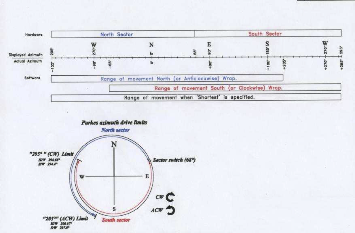
The antenna follows a source for a specified duration; it is possible to do this from the source rising to setting with the elevation limit defined by 30.25 degrees. The only limitation is where the antenna drifts into either the upper Zenith limit past 1.12 degrees, or the Azimuth wrap limits at 205 or 295 degrees. The Azimuth wrap limits are defined in Figure 1.10 below.
The Drift mode is an extension of Track. Using specified coordinates, the antenna is driven to an offset position, which is -(duration/2) seconds (of time) before the given position. Once there, a secondary calculation is done to determine the Azimuth and Elevation and the antenna driven to these coordinates and tracks there for duration seconds. Whilst the Azimuth and Elevation are fixed for the observation, other coordinate systems (B1950, J2000, GALACTIC) become epoch of date.
Grid mode is an extension of Track. The telescope tracks each position in a grid of observations. This allows the antenna to create an l (1D) or l x m (2D) grid of positions, with an optional reference position to be revisited every nth observation. Currently, there is no specific mode to create point grids with Dhagu?, it is possible to define reference and/or on-source positions manually.
The telescope is able to scan between two selected endpoints, at some desired rate (i.e., 3 deg/min). A series of scans can be merged together to create a map. Dhagu? currently allows maps to be defined as on-the-fly (OTF), where scans are observed in turn, with the bandpass calibration is performed by using the scan data itself. There is also the option of performing referenced scanning, where a reference point outside the map region (presumably free of emission) is observed for a short time. Interleaved scans are observed before returning to the reference position. Scans can be done along a small (i.e., parallels of latitude) or great-circle path. The hard-coded definition of a small-circle scan is where the latitude of the start coordinate was exactly the same as the latitude of the end coordinate; otherwise a great-circle scan is done. Please also note scanning within 10 degrees of the upper Zenith limit is not recommended and should be avoided to reduce antenna structural stress and active the anti-vibration proceedure of the Telescope Protection System (Section 3.1.2.6), which will stow the antenna.
SPOT is a position determining mode which does a number of RA and DEC scans to determine the best position of a source. Its primary use is for pointing, though it can also be used to determine source fluxes relative to the calibration waveform, and obtain accurate beam parameters such as the FWHM. Only continuum mode is supported.
If the telescope is wind parked, stowed or not able to be driven, but all other subsystems are available, the NoDrive template can be used. In this mode, the antenna drives are not enabled and observing can take place with the sky passing through the receiver's field-of-view, at the sidereal rate. As with the Drift mode, whilst the Azimuth and Elevation of the antenna remain fixed, other coordinate systems (B1950, J2000, GALACTIC) are epoch of date. This mode would be useful for FRB transit detection surveys with the CryoPAF.
Observers should avoid putting undue stress on the drive systems of the telescope by avoiding tracking a source through Zenith. A warning is sounded in FROG when an observation moves within 5 degrees of Zenith, but observers should take precautions to avoid tracking a source within a couple of degrees of zenith (sources with declinations of approximately -30 to -32). Not only does it put stress on the drive systems, but it will also likely result in poor data as the telescope struggles to maintain tracking lock. As such we request observers to be conscious of these limits and schedule sources appropriately. If only one source is being observed, and it tracks within a couple of degrees of Zenith, observers should stop observing, wait for the source to transit, and then restart observing.
With the transition to web-based observing, it is not possible to support every web browser on every platform. As a result, whilst observing with Murriyang should be possible with any modern up-to-date browser (i.e, Firefox, Microsoft Edge, Google Chrome, Safari Opera, ...), we officially support browsers/versions as per below. There is a simple browser check in most web apps with a prompt appearing at login if the browser appears to be unsupported. If you are running an unsupporeted browser, the application will not load. For this reason, it is stongly recommended you check your browser well in advance of your scheduled observations. If the check appears incorrect, please submit a report via the Links -> Fault Reporting page on the PORTAL.
Whilst our applications use mobile device frameworks such as Bootstrap, we do not officially support viewing or running any application on a mobile device.
To assist with debugging efforts, it would be useful to include in a ticket (email to parkes.support[at]csiro.au) the operating system and version, plus browsers/versions used. To ascertain if the issue is network or client related, please include any output from the browser Web Developer, or JavaScript consoles; please check your browsers' help menu on how to display the console. It is important to accurately describe the issue; if you find an application "slow", does that imply the UI refresh rate is poor, with updates not being displayed as expected, or is it definitively a network issue? In recent times Firefox users have reported high CPU/memory issues, so if you are experiencing issues running an application with Firefox, please indicate any GPU/CPU intensive aplplications running at the same time, if any. If avaialble, please include any dependancy versions listed under the "Help" tab of the application..
Please note any issues reported must be with a supported browser.
Table 1.12. Supported web browsers.
| Browser | Version |
|---|---|
| Firefox | 78+ (Debian Linux), 82+ (Macintosh) |
| Google Chrome | 86+ |
| Microsoft Edge | 86+ |
All observers will need a CASS Unix account and password in order to access the various observing tools and utilities.
This is an essential element of remote observing.
If you do not have one already, then you can apply to get one here. It usually takes a week or two for the request to go through the system. Therefore, it is important that you put in your request for a Unix account at least a week before your scheduled observations. Similarly, if you have an account already, but it has lapsed, then you will need to send an email to atnf-ci[at]csiro.au at least a week ahead of your observations to reset your password.
Various tools exist to help you plan your observations. A full list of tools can be found on the Murriyang Observing Information web page (look under “Planning your observations”): here.
Below are some of the more useful tools.
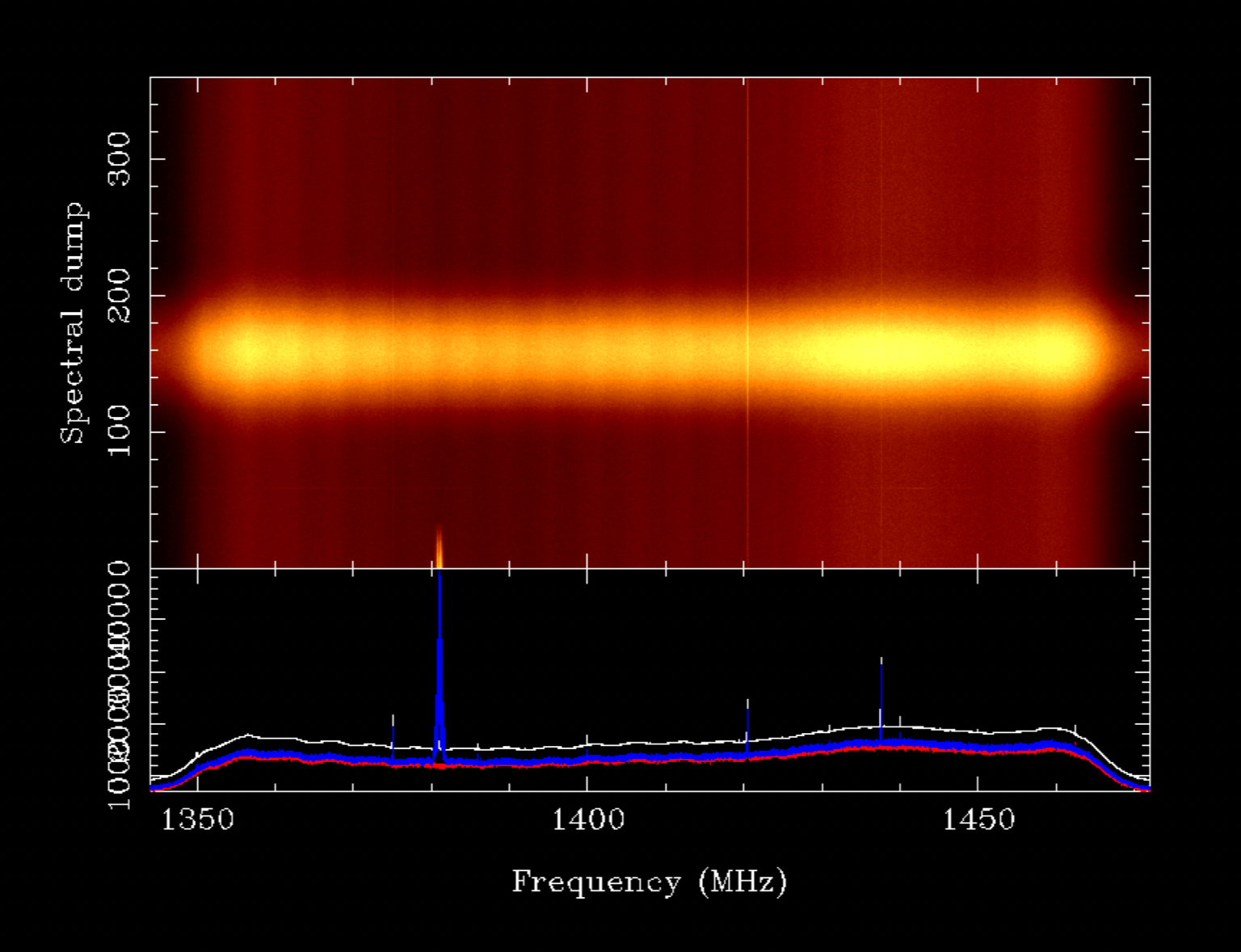
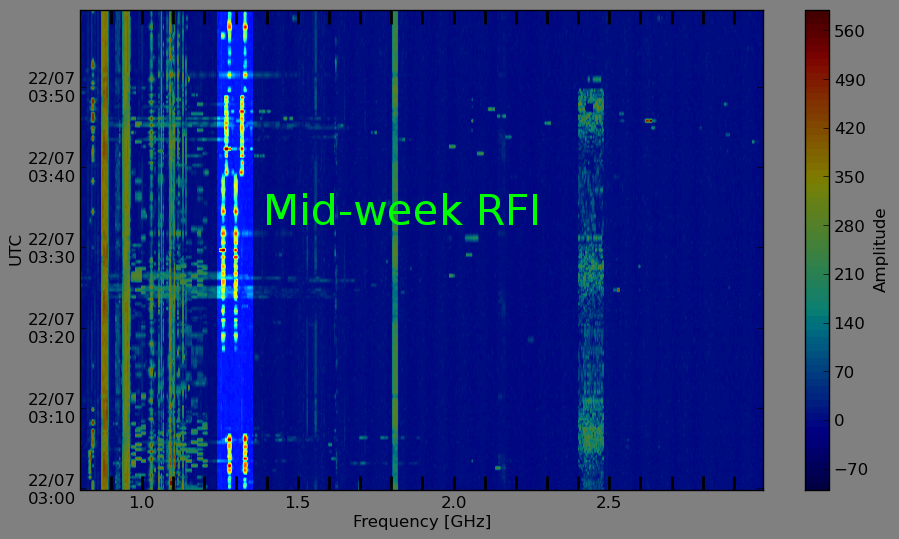
The PORTAL includes information (under ‘alerts’) on any particular forecast RFI - this is typically at L band and may be unavoidable but should there be flexibility in the observing strategy, one mitigation is to observe at a different part of the band or with a different receiver (if for example a high frequency receiver is installed). This RFI has frequency peaks around 1265 and 1300-1310 MHz, and can have extremely high amplitudes. The RFI monitor (see below) can be used to see when mid-week RFI is present, as shown in Figure 1.13 Because of the strength of this RFI, it can often drive the front-end system into saturation; if this occurs, the data becomes unusable. We do now sometimes receive advanced warning on when this RFI may be present, and if this will affect observations, the notification will be made on the PORTAL and possible alernative arrangements, such as switching receivers and/or frequency can be made.
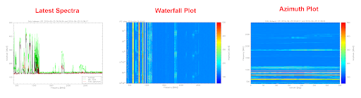
The Parkes Observatory has a real-time RFI monitoring antenna that is located on a tower, a few hundred metres to the East of the telescope. It is a log-periodic antenna and is used to measure and identify the many man-made signals that are produced by on-site and off-site sources. The antenna scans the site, completing a full circuit every 20 minutes. Every 20 seconds the data is updated and displayed on the web site linked below. It monitors the frequency range 700 - 3000 MHz with 2 MHz frequency resolution. The data is presented in three different format:
A power spectrum of the “latest spectra”. It is zoomable by moving the cursor over the spectrum.
The spectrum as a function of time in the form of a waterfall plot showing the last hour of data.
The spectrum as a function of azimuth.
The RFI Weathermap is avaliable here.
Many satellite constellations regularly transmit in our receiver observing bands. The best way to deal with them is to avoid them all together. On the sky plot of FROG (or Dhagu?), you can display the satellite constellations that are known to transmit in your observing band and then avoid those parts of the sky populated by the satellites.
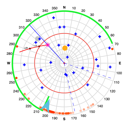
Figure 1.15. An example of the sky plot on FROG showing the GPS Satellite constellation (NAVSTAR) as blue crosses.
The UWL system and the MEDUSA backend potentially allows for extensive data rates that can impact other observers and the ability to take further data. As such we ask that observers clearly stipulate their expected data rates on their observing proposals and maintain those for the actual observations. The Dhagu? system will check the data volumes exceed 0.5 TB.hour, notifying observatory staff if exceeded. In general, the scheduler will endeavour to ensure data intensive projects are not scheduled too close to one another, but this cannot be guaranteed.
To calculate data volumes with the UWL:
- Pulsar Search: File size [bytes] = Nchan x Npol x Nbit/8 x Tobs/Tsamp
- Pulsar Fold: File size [bytes] = Nchan x Npol x Nbin x 16/8 x Nsub
- Spectral line mode: File size [bytes] = Nc_sb x Nsb x Npol x Tdump x 32/8
- Voltage Capture (non-standard): File size per zoom band [bytes] = Nbit/8 x BW x 1e6 x 2 x Tobs x 2
where:
- Nc_sb = number of channels per subband
- Nsb = number of subbands (normally 26 for the UWL)
- Nsub = number of subintegrations in pulsar fold mode
- Nchan = total number of channels = Nc_sb * Nsb
- Npol = number of polarisation states (1, 2 or 4)
- Nbit = number of bits/sample (1, 2, 8, 16 or 32)
- Tobs = observation time (seconds)
- Tsamp = sampling time (seconds)
- Tdump = number of spectral dumps (the total integration divided by the sampling time (seconds))
- BW = bandwidth in MHz
Noting that the total data volume will be a few percent larger than that given by the equation because of the need to store meta-data information. Also, note that Dhagu? will calculate the data rate when a Parameter Set is displayed via the Show parameters button under the Editor tab. In addition, the rate is also shown when you update or save a Parameter Set. If the calculated rate is in excess of 0.5 TB/hour, data management will be notified.
In general to observe with Murriyang you must submit a proposal to the ATNF Time Allocation Committee via the OPAL webpage (https://opal.atnf.csiro.au). There are exceptions to this (purchased contracted telescope time and targets of opportunity). A proposal consists of a cover sheet, a table of observations and a science case. Calls for proposals are made every 6 months (in approx. June and December), with meetings of the Time Allocation Committee thereafter (typically in July and February respectively). Proposals are allocated a project code on submission of the form of a ‘P’ followed by an iterative 4 digit number (previously 3 digits). Exceptions to this convention are contracted time (given a name for example ‘BL’ or a special code for example PX500 and PX501) and Target of Opportunity observations (also PX but with a 3 digit number much less than 500). Proposals are graded by the committee and then those with sufficient grades will be allocated some or all of their requested time (typically grades of at least 3.0 are required, and time will be scheduled in the subsequent semester, starting October or April respectively). Scheduling is a function of the proposal pressure and requested Local Sidereal Times, meaning that exact allocations, and grading cut-offs, vary from semester to semester. If you are unable to find your project code during the setup for your observations, use the code `PUNDEF’ and contact support after your observations to reassign the correct code do your data.
The Parkes Observatory operates a model whereby each project should have a designated ‘Observing Expert’. These individuals should be trained in the use of Murriyang, qualified to observe remotely and available to assist the project with any scientific or observing strategy related queries. They are also expected to train their team members in any specifics to their projects (separate to the basic remote observer training provided by the national facility). If the proposal team does not include someone who is already qualified then the team must send someone to visit the ATNF and receive appropriate training (or recruit an expert to their team). The Observing Expert is expected to be present with any first time observers to provide assistance as required. The Observing Expert should be identified on the OPAL proposal cover sheet.
Successful proposals provide clear and succinct science cases that motivate the proposed observations. They identify why the observations should be carried out with Murriyang (and not another facility) and demonstrate that the proposers have appropriately considered what is required to achieve their science goals. The OPAL proposal cover sheet allows for the selection of the preferred receiver and backend. The default receiver pairing is the UWL and a high-frequency receiver such as 13MM or MARS. If another receiver from the fleet is required this should be clearly motivated and will require a substantial time request and high Time Allocation Committee grading to instigate a change of receivers from the default pairing. Alternatively observations with other receivers can be entertained if combined with the VLBI observations for the semester (for which proposers should liaise with the LBA System Scientist).
In addition to standard scheduled observations there are two types of observation that can override the schedule:
These are proposals of a non-claim-staking nature for a well-defined set of observations but requiring specific dates and times for observations that are not yet established. This is either because they are in response to a trigger which is unpredictable in time, or because they are a component of commensal observations with another facility with a different timeframe for allocation to that of ATNF proposals. The proposal is submitted to OPAL as usual, but identified as a Non-Apriori Assignable Proposal (NAPA) in the system. The proposal is then assessed by the Time Allocation Committee as usual, receiving a grade, but is only scheduled on the telescope when an event is triggered or commensal observations scheduled. If triggered they may displace any lower ranked proposal at the discretion of the scheduler.
These are unexpected astronomical events of extraordinary scientific interest for which observations on a short time scale are justified, and for which a NAPA was not possible (i.e. the request was unforeseen). To trigger such an observation requires an email to the scheduler and to the alert email address. Your email should include a scientific justification (of order half a page to one page) providing sufficient technical detail for the observations to be scheduled. These observations are allocated a number of the form of a ‘PX’ followed by 3 digits.
Time unallocated in the semester schedule, which is elsewhere often referred to as ‘Director’s Discretionary Time’, is referred to within the ATNF as ‘green time’ (due to the green hue in the graphical schedule, example below).
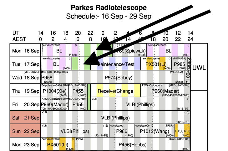
Traditionally this time would have been requested via an email to the ATNF Director, or Head of Science Operations, but is now through the PORTAL and an email to the scheduler. This should include information on the proposed observations, a rationale for the request, and any project codes that may be relevant (for example if you are asking for additional time for a scheduled project, time would be allocated to the same project code).
Instrumentation enables various calibration strategies. The primary calibration goals are to:
- Ensure the telescope is pointing accurately
- Remove fluctuations and ripples in the bandpass
- Scale astronomical sources to flux density units
- Account for gain fluctuations throughout the observation
- Form calibrated Stokes parameters for the astronomical sources.
Pulsar astronomers generally observe a switched calibration signal prior to the pulsar observation. Spectral line/continuum observers have made use of a wider range of calibration strategies including position and/or frequency switching, pointing models, beam switching and calibration signals. Bandpass ripples also need to be accounted for during data processing.
We note that the fixed digitisation for the UWL receiver precludes frequency switching calibration systems for observations with that receiver.
The UWL receiver and other legacy receivers within the fleet enable the injection of a switched noise source into the signal path. Typically this switched calibration system is used as follows:
- Pulsar fold-mode observations: the telescope is pointed a few beam-widths away from the source of interest and the switched calibrator run with a 50% duty cycle and a frequency of 11.123 Hz. A fold-mode observation is recorded (typically with the source name being <pulsarName>_R. The calibration signal is then switched off during the pulsar observation.
- Pulsar search-mode observations: traditionally, no calibration signal is applied for pulsar search observations. For studies of single pulses from known pulsars, then the calibration signal is switched (as above) prior to the start of the pulsar observation.
- Spectral line/continuum observations: the calibration signal can be applied continuously during the observation or for a specified short observation In this mode, the UWL backend instrument produces a cal-ON and a cal-OFF spectrum alongside the higher resolution astronomy spectrum. It is typically switched with a 50% duty cycle and a frequency of 100 Hz.
A characteristic small-scale ripple with a periodicity of 5.7 MHz arises from multiple reflections in the 26m space between the vertex at one end, and the focus and/or underside of the focus cabin at the other. Analysis of the UWL spectra also shows small-scale ripples on a range of periodicities and these are actively being studied with the goal of their removal. The primary 5.7 MHz ripple is usually mitigated in offline processing by baseline fitting, or position switching, but it is also possible to cycle the (high frequency) receivers up and down in the translator Y-axis to ‘smear out’ the ripple with amplitude 6.3mm peak-to-peak and a period of 60 seconds. This technique is available for use with higher-frequency receivers only and proposers should contact operations, ATNF-Parkes-Remobs[at]csiro.au before submitting proposals.
Flux calibration sources in the Southern Hemisphere can be identified from the ATCA calibrator database. Flux density calibrators that are commonly used are listed below:
Table 2.1. Standard Calibrators.
| Source | RA J2000 | Dec J2000 | Notes |
|---|---|---|---|
| PKS 0823-500 | 08:25:26.869 | -50:10:38.49 | f < 10 GHz; ATNF Standard flux calibrator. |
| Hydra A (3C 218) | 09:18:05.7 | -12:05:44 | f < 3.5 GHz. |
| PKS 1253-055 | 12:56:11.166 | -05:47:21.52 | f > 10 GHz; variable, tie to ATCA flux. Occulted by Sun around 8th Oct. |
| PKS 1934-638 | 19:39:25.026 | -63:42:45.63 | f < 10 GHz; Primary ATNF Standard flux calibrator. |
| PKS 1921-293 | 19:24:51.056 | -29:14:30.12 | Variable, tie to ATCA flux. |
Most observing projects obtain their own flux calibration solutions. However, the switched calibrator source is relatively stable for the UWL, so flux density calibration solutions taken within weeks or months of a particular observation are generally sufficient for use (assuming that the switched calibration signal is used).
Cross coupling in the feed was a major issue for the 20CM Multibeam receiver. In Figure 2.1 below (Kerr et al. 2020) we show, for different receivers, the ellipticities of the receiver system and as well as the orientation of receptor 1 with respect to receptor 0 (). In brief, the co-axial 40/50 cm (left) and 10 cm systems (right) are close to the ideal feed assumption over most of the band. The 20CM Multibeam system (middle) shows substantial non-orthogonality and cross-polarisation, while the 20cm H-OH feed is also close to ideal.
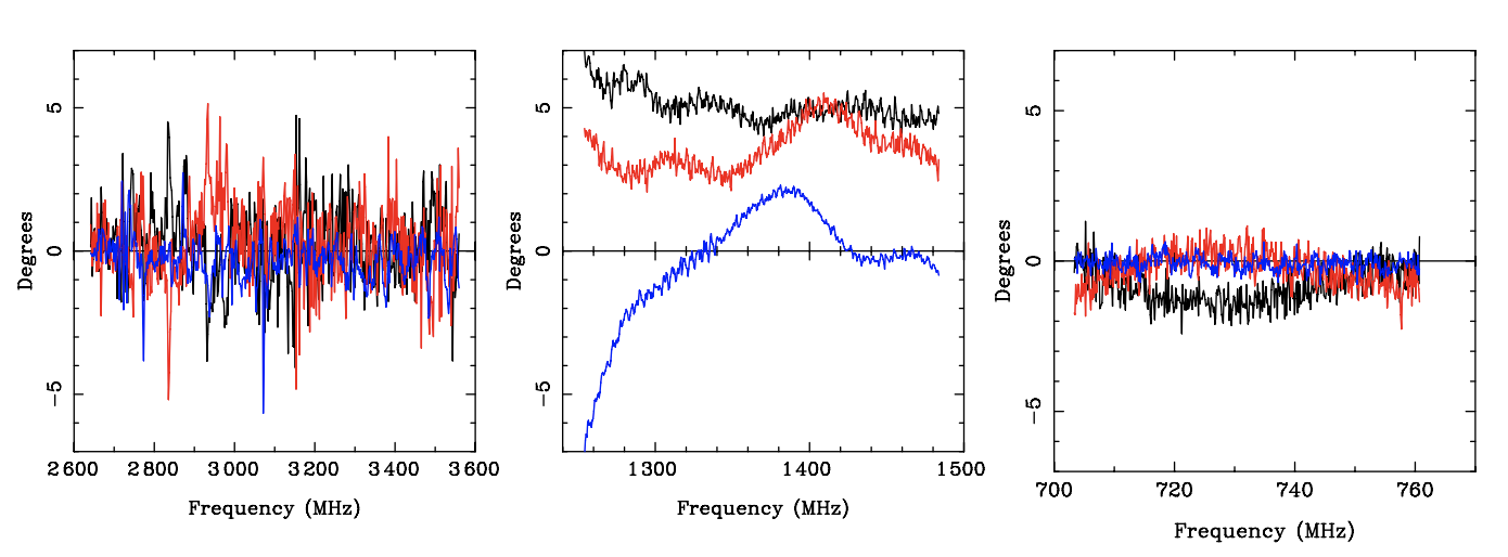
For the UWL system, the measured receptor ellipticities are close to 0 degrees across the whole band, indicating that the degree of mixing between linear and circular polarisation is low. The non-orthogonality of the receptors is also very low. At higher frequencies, the reference signal produced by the artificial noise source deviates from 100% linearly polarised. Up to ~30% circular polarisation has been observed at ~4 GHz and this must be accounted for in the offline processing.
The P737 observing project carries out rise-to-set tracks of the bright, millisecond pulsar, PSR J0437-4715 approximately once per semester with the UWL receiver. These observations can be used to track any changes in the cross-coupling parameters within the receiver system.
The basic requirement of scheduling an observation with Dhagu? is the Parameter Set. This is a list of key/value pairs which configure the TOS and MEDUSA subsystems. Once a Parameter Set is created, it can be submitted to TOS, which then creates a Scheduling Block. A Scheduling Block is an atomic entity (unique number) and contains all the information on the requested observations. Each Scheduling Block has an associated state, which reflects the status of the observation before (DRAFT, SUBMITTED, SCHEDULED), during (EXECUTING), or after (ERRORED, OBSERVED) the Scheduling Block has been submitted to the Observing Queue.
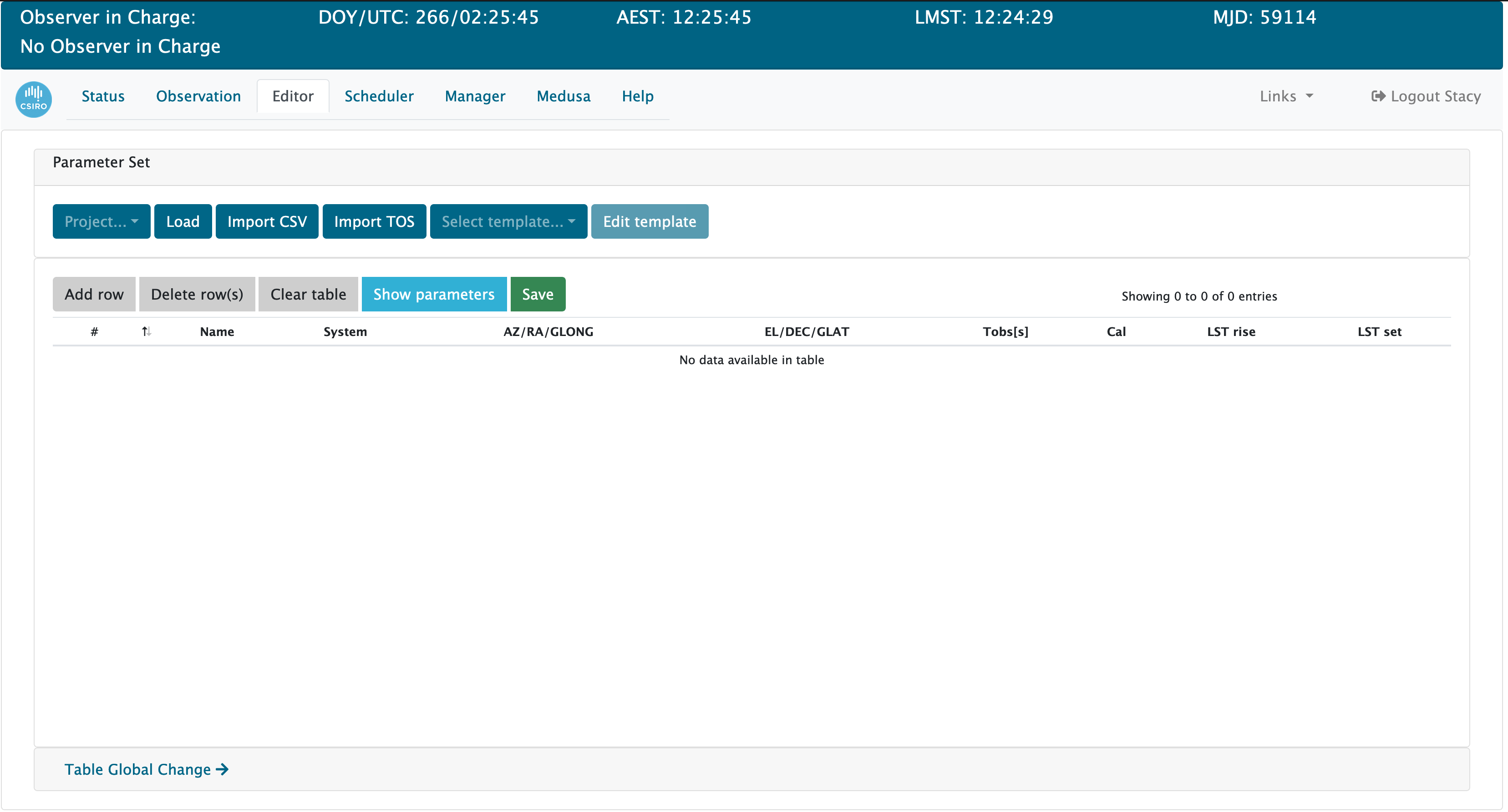
There are several ways to create a Parameter Set in Dhagu? From the Editor tab shown below in Figure 2.2, you have:
- ability for direct entry of sources via the editor table, though first you configure MEDUSA first (via Select template...).
- ability to upload a Comma-Separated Values (CSV) source list, and configure MEDUSA manually (via Select template...).
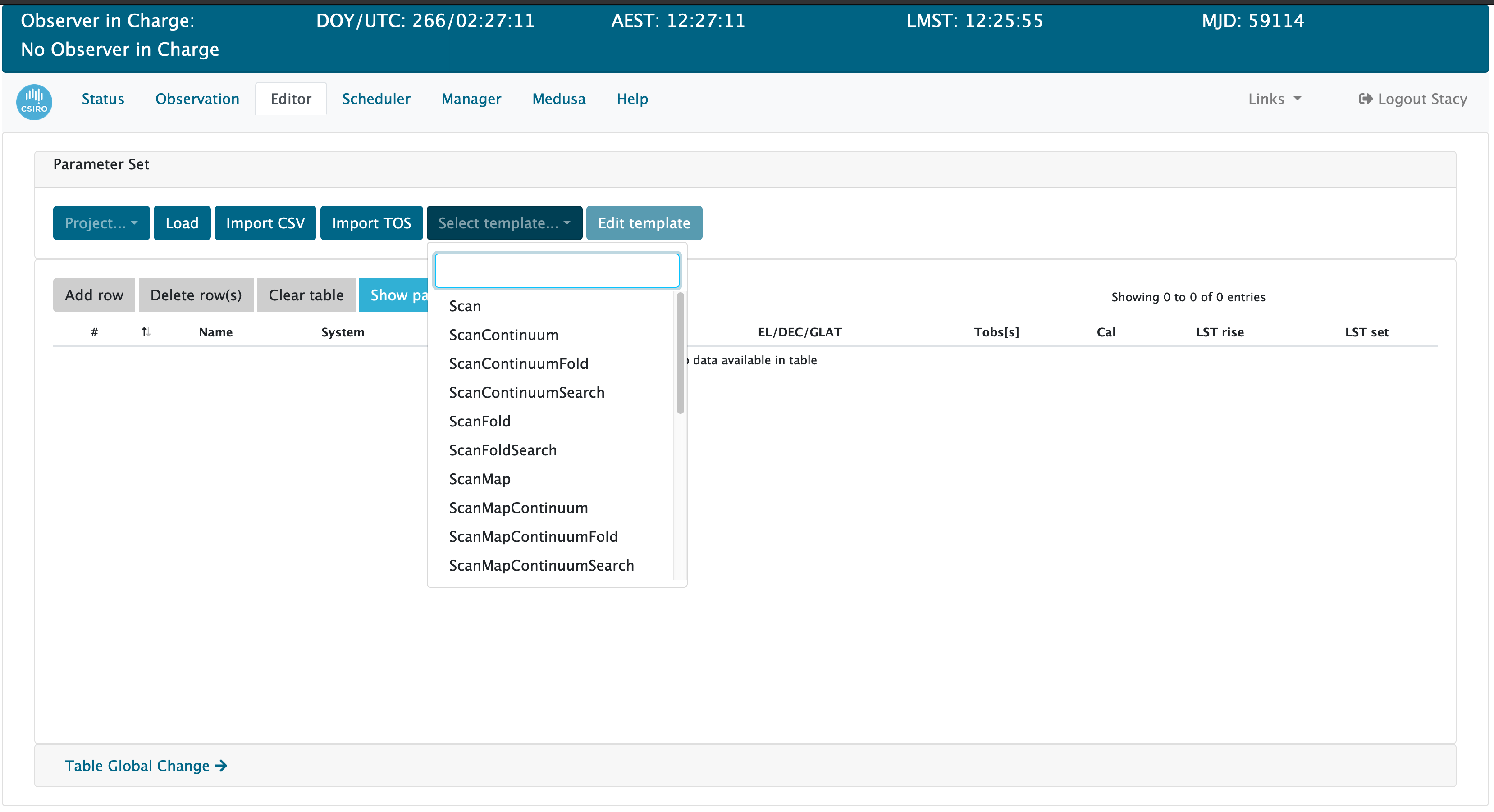
Before you start entering sources manually, you must first select the configuration you wish to use from the Select template... dropdown menu (see Figure 2.3). When the selected option is clicked, the MEDUSA configuration tool (Section 2.4.3) will apprear. The Track, Scan and ScanMap options do not have a MEDUSA configuration, which is useful if you want Dhagu? to drive the antenna and calibration waveform, but drive MEDUSA manually. If you select a ScanMap* option, you will also need to define the map parameters (widths, spacing, direction, etc...); the chosen options will auto-populate the scanning start and end positions in the Editor table. Once you are happy with the selected configuration, click the Save button.
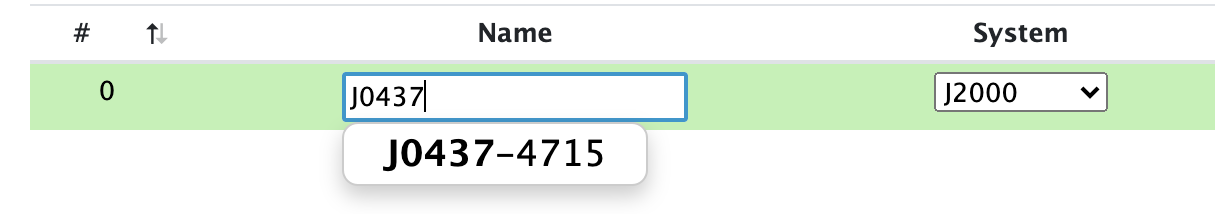
You can now add sources into the Editor table. For reference positions in a ScanMap configuration, it will only have the tracked position, whereas the scanning rows will have a start and end position. To add sources to the Editor table, click on the Add row button. For the source input, a typeahead exists which is linked to the PSRCAT and ICRF J2000 catalogues. These present the observer with a list of matching sources (maximum 10 listed) to select from as shown below. When a source is selected, the name, frame (J2000), RA, DEC and LST Rise/Set fields are populated automatically.
You can add or remove rows, or clear the table. The Clear table button does not touch the calibration waveform or MEDUSA configuration. To clear these, simply reselect the template from the dropdown menu, and click the Reset button at the bottom o the modal popup.
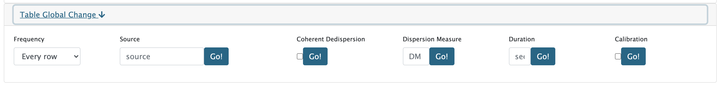
It is also possible to auto-populate rows using the Table Global Change section, as shown above in Figure 2.5. By clicking Add row, the observer can add (say) 10 rows to the table, then in the Table Global Change section, enter their PSRCAT or ICRF J2000 source only once, and click Go! All rows, whether every row, of the nth row of the table (n < 10), should now be populated with the chosen source. Similarly, if the observer wishes to populate the on-source duration (seconds) or toggle the calibration waveform, it can be done here. It is not currently possible to pass names to an external query database like Simbad, but this may be added in the future.
TOS accepts coordinates in J2000 or AZEL only. However, Dhagu? allows J2000, AZEL and GALACTIC. When the Show parameters or Save buttons are pressed, coordinates are converted to J2000 if GALACTIC is selected. If you need accounting of Galactic coordinates in some way, use the longitude/latitude in the name of the position, ie., G200-2.5.
You can reorder sources by using click+drag on the first column to its destination. You can also reorder sources with more flexibility when loading the saved Parameter Set into the Scheduler, or the Pending list of sources. Once done adding sources, you can save the table as a Parameter Set clicking Save.
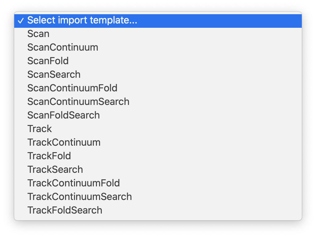
By clicking the Upload CSV button, you can select and import a CSV file. The list of options is shown below. You define the observation import template of the CSV file by clicking Select import template. Then click Browse, your OS will present a finder window, which will allow you to select a CSV file to upload. Once you have selected a file, the filename will be present in the entry box adjacent to the Select button. By clicking the Upload button, the process of uploading and parsing the file will begin. In the event of errors in parsing the CSV file, only the first five (5) error messages will be displayed.
The format of the import is defined by a header in your CSV file, which must be present. For TRACK, the full header list is as follows:
name,x,y,frame,duration,cal,comment
Here, x and y are source coordinates determined by epoch, where GALACTIC implies x = longitude (degrees) and y = latitude (degrees). You can also add a comment for the source as the last column.
For SCAN observations, the full header list is as follows:
name,x,y,frame,scan_length,scan_rotation,duration,cal,comment
Here, the name, x, y, frame, duration and cal keywords have the same meaning as for Track observations. The scan_length paramter allows the scan length to be determined (degrees), orientated at angle scan_rotation (degrees). The rotation angle is positive for a clockwise rotation. A rotation angle of 0 degrees implies the scan will proceed from North to South. You can change the direction of the scan by specifying a negative direction. As with TRACK observations, the comment parameter allows you to add a comment to this source.
If the object name is contained in the Pulsar PSRCAT or ICRF databases, the import process will generate the J2000 coordinates and auto-populate these in the table. Therefore if you are using sources from these catalogues, the minimum set required for Track is name and duration, and name, scan_length, scan_rotation and duration for Scan. Keywords can be in any order, but must match the header. If your sources are not in PSRCAT or ICRF catalogues, you will need to supply the x/y coordinates and frame, or the source will be skipped during the import process. A source will also be skipped if the ephemeris indicates the source will never rise above the horizon. The import process will attempt to minimum match source names to PSRCAT and ICRF sources if the coordinates are not present. An example Track CSV file is shown below:
          name,x,y,frame,duration,cal
          J0437-4715_R,04:37:16,-47:00:00,J2000,30,true
          J0437-4715,,,,180,false
The first source is a provided reference position, which has the _R extension; this is not mandatory, only historical for denoting a reference position. The reference is located to the North of the given Pulsar position, with the calibration waveform switched on for 30 seconds. The second source is the catalogue Pulsar position proper, and the calibration waveform switched off and integrating for 180 seconds.
An example Scan CSV file is shown below:
          name,x,y,frame,scan_length,scan_rotation,duration,cal
          1934-638,,,,1,0,600,false
          1934-638,19:39:25.026661,-63:42:45.62554,J2000,1,135,600,false
The first line defines the header. The second line is a one degree scan across PKS 1934-638 with a rotation angle of 0 degrees, resulting in a North-South scan. The coordinates for PKS 1934-638 will be populated via Dhagu? The next line is again PKS 1934-638, with coordinates defined and another one-degree scan but at a rotation angle of 135 degrees, clockwise from North. For more information, see the Scan example in Section 2.11.
Caution
Importing a CSV file will not alter the MEDUSA configuration at all. If you have configured (say) the TrackContinuum configuration, once you have imported your CSV, clicking on Show parameters will show that configuration attached to your CSV input. This is to allow importing multiple CSV sets with the same MEDUSA configuration.
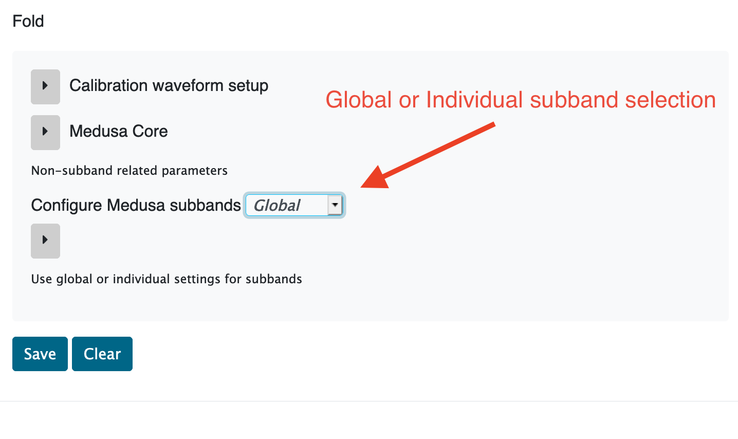
The MEDUSA configuration tool is a form that allows you to change parameters sent to the MEDUSA backend. It is available from the Select template... dropdown menu. If you have loaded parameters, you just also use the Edit template button. Depending on the required antenna and MEDUSA mode, the form will be different, but as an example, the TrackFold form is shown below in Figure 2.7. MEDUSA parameters are grouped by functionality, and for some configurations such as commensal modes, there are quite a number of parameters, though you are not necessarily required to view and modify all of them. Clicking on the > buttons to expose settings that may need to be configured. The provided defaults for all modes configure MEDUSA to display data across all subbands and provide a good starting point for refinement, according to project specifications. The Calibration waveform setup dropdown in Figure 2.7 is the waveform control, where you can set the frequency, phase and duty cycle of the calibration signal. The Core dropdown allows you to configure properties for all subbands such as how the system temperature is calculated. Individual modes such as Fold will have other parameters in this section.
The Configure subbands dropdown allows you to configure MEDUSA subbands in one of two ways, global or individual. With global settings, you apply a single set of parameters to selected subbands. There are convenience options to select the low (0-4), mid (5-12) and high (13-25) subbands of the UWL receiver with the click of a button. If you want to have different configurations (i.e., number of channels) for selected subbands, the individual option is provided. For example, a spectral-line observer would only select subband 5 if only interested in Galactic HI, subband 7 for the Hydroxyl (OH) transitions at 1612, 1665, 1667 and 1720 MHz, or subbands 0, 19 and 20 to observe all transitions of Methylidyne (CH) at 701, 704, 722, 724, 3263, 3335 and 3348 MHz. To add and configure subbands, click on the + button.
Once satisfied with the MEDUSA configuration, the Save button.
Caution
Clicking the Save button in the MEDUSA configuration tool only saves that configuration within the browser. To save the MEDUSA AND source-related parameters to disk, you need to use the Save button atop of the editor table.
With MARS and 13MM receivers now added into Dhagu? (since v2.0), setting up a Parameter Set requires extra consideration given these receivers still require the legacy tower digitizers, conversion system and switch matrix. In the past, observers would need to run an "lorun" and "smrun" script in the joffrey:1 VNC. Whilst this process is still required, it is now done automatically by TOS. For the switch matrix, given the maximum bandwidth of the conversion system is 1024 MHz, this is the default and allows for 8 x 128 MHz subbands. For the MARS receiver (7900 - 9100 MHz), this covers the entire bandpass, but for 13MM (16000 - 26000 MHz), the whole bandpass must be covered by seperate configurations.
Caution
It is not possible to dynamically set the on-sky frequency.
Caution
The lorun scripts used by TOS are NOT located on joffrey.
The following MEDUSA setups are offered; contact Parkes Operations for other options.
Table 2.2. MEDUSA Setups for MARS/13MM
| Receiver | Sky freq (MHz) | Total BW (MHz) | 128 MHz Subbands | MEDUSA | ConvSys |
|---|---|---|---|---|---|
| MARS | 8457 | 1024 | 8 | apollo.mars | mars_8457.cmd |
| 13MM | 17500 | 1024 | 8 | apollo.13mm_17500 | 13mm_17500.cmd |
| 13MM | 22235 | 1024 | 8 | apollo.13mm_22235.cmd | 13mm_22235 |
Note the sky frequency above is actually the center frequency of subband 3 (zero based.).
An example of setting up a Parameter Set with the MARS receiver to observe a Pulsar with Dhagu? is shown in Section 2.12.
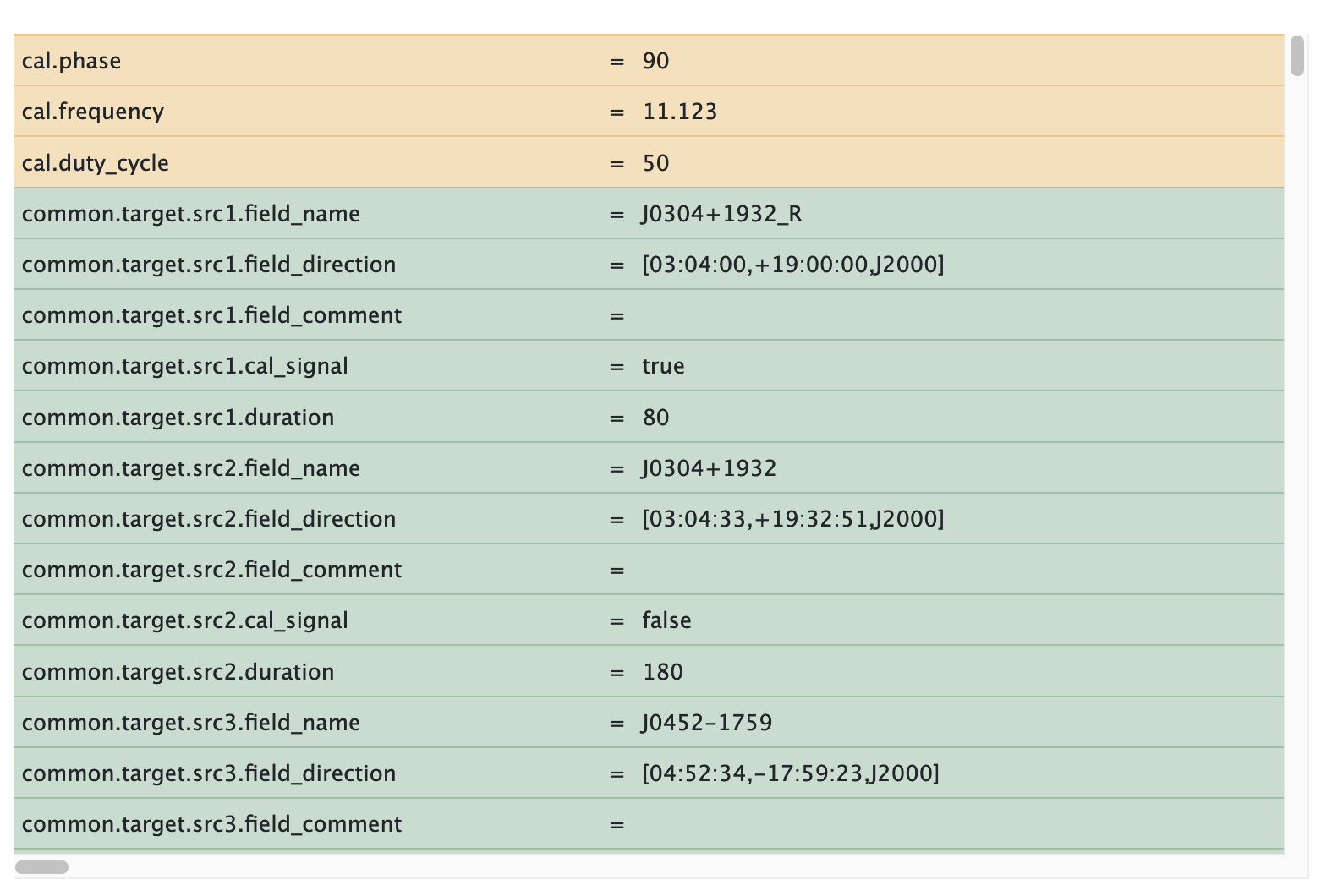
Once the source and MEDUSA parameters have been set, the observer can display the entire Parameter Set before saving, as shown in the example below. Parameters in green are TOS, and those in blue are MEDUSA parameters in orange represent other hardware components. Once the parameters look fine, dismiss the popup and select (if not already) the project to associate the parameter set with, but using the Project button, then click on Save. A secondary popup will prompt for an alias, which is a alpha-numeric string, something to distinguish this Parameter Set from others. You can view the saved parameter set from the Manager tab, or (re)load it into the same table or load it into the Scheduler tab for submitting sources for observing.
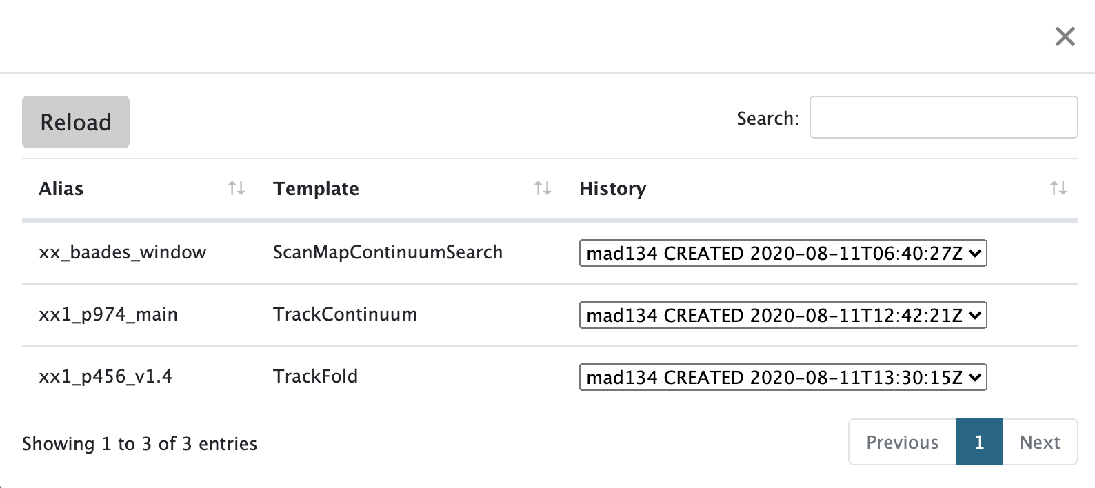
Once you have saved Parameter Sets in Dhagu?, you can easily load them back into the Editor table. First, select the project the Parameter Set was saved to, using the Project... button above the editor table. Next, click on the Load button, and a list of saved Parmeter Sets should be diplayed. The table columns are sortable by clicking on the column headers. The table (example below) shows the ID of the Parameter Sets, the template (TrackFold, TrackContinuumSearch, ...) and a history with a dropdown menu showing who made changes and when (UTC timestamp.)
Caution
There is no revision control of Parameter Sets in Dhagu?, although there is a history of changes as shown in Figure 2.9, though each Scheduling Block contains the Parameter Set used to run the observation, so past versions of a Parmeter Set can be viewed and/or copied via the Manager tab if required. By clicking on a row, the selected Parameter Set will be loaded into the Editor table, where it can be altered and either saved as a new Parameter Set (define a new alias when saving), or if the alias is the same as a pre-existing one, it will replace the existing one.
An existing TCS FOLD mode observation with the UWL receiver and PDFB4 may look like the following, which utilised the low (768MHz; CASPSR) and high bands (>3100MHz; PDFB4) of the UWL (this would all be on one line to be read by TCS):
        J0835-4510_R; P 08:35:00 -40:00:00; d4_cfg pdfb4_1024_1024_1024;
        d4_frq 3100.0; d4_tcyc 10; d4_tsub 30; rcvr UWL; tobs 120;
        mode levcal; cal freq; cfrq 11.123; fdmode FA; fdang 0.0;
        MED_PROC FOLD128; MED_SUB 30; MED_BIN 1024; MED_CHN 1024;
        CA_PROC dspsr.50cmsktoo; CA_FRQ 724.0; CA_BW 64;
The above TCS schedule equates to TOS/MEDUSA Parameter Set as below. Whilst more verbose, fine-grained control of subbands is possible via TOS, but not TCS. As we are selecting specific subbands, we disable all subbands first (using apollo.fold.subband%d.active) and specify (activate) those we want. For MEDUSA, subband0 equates to 768 MHz with 127 MHz bandwidth (equivalent of CASPSR), and subbands 13-20 cover the 3100 MHz, 1024 MHz bandwidth used with PDFB4. In the example, Kurtosis RFI Mitigation is turned on for subband 0 only; setting subband%d.enable_sk to false disables all other subbands.
        cal.frequency = 100
        cal.duty_cycle = 50
        cal.phase = 90
        common.target.src1.cal_signal =  true
        common.target.src1.duration   =  30
        common.target.src1.field_direction  = [08:35:00,-40:00:00,J2000]
        common.target.src1.field_name =  J0835-4510_R
        common.target.src2.cal_signal =  false
        common.target.src2.duration   =  120
        common.target.src2.field_direction  = [08:35:20.61149,-45:10:34.8751,J2000]
        common.target.src2.field_name =  J0835-4510
        common.targets = [src1,src2]
        apollo.fold.subband%d.active =   false
        apollo.fold.subband%d.enable_sk = false
        apollo.fold.subband%d.output_nchan = 1024
        apollo.fold.subband0.enable_sk = true
        apollo.fold.subband0.active  =   true
        apollo.fold.subband13.active  =  true
        apollo.fold.subband14.active  =  true
        apollo.fold.subband15.active  =  true
        apollo.fold.subband16.active  =  true
        apollo.fold.subband17.active  =  true
        apollo.fold.subband18.active  =  true
        apollo.fold.subband19.active  =  true
        apollo.fold.subband20.active  =  true
        apollo.fold.subband21.active  =  true
Caution
Specifying the DM or period is not required if the source is in PSRCAT. A value of -1 for the DM will ensure MEDUSA applies the PSRCAT values. For a new Pulsar that is not in PSRCAT refer to Section 1.7.1.1.
An existing TCS Search mode observation with the UWL receiver and PDFB4 may look like the following, with Stokes I (AA+BB) only (this should all be on one line to be read by TCS):
        J1227-6230; P 12:27:39.96 -62:30:19.2; mode srch; tobs 3600;
        SR4_FTMX 900; pid P860; MED_PROC SRCH; MED_POL 1; MED_CHN 128;
        MED_BIT 8; MED_SMP 128; MED_DM 100.0; MED_SUB 15;
The corresponding TOS Parameter Set is:
        cal.duty_cycle = 50
        cal.frequency = 11.123
        cal.phase = 90
        common.target.src1.cal_signal = false
        common.target.src1.duration = 3600
        common.target.src1.field_direction = [12:27:39.96 -62:30:19.2, J2000]
        common.target.src1.field_name = J1227-6230
        common.target.src1.search_co_dedisp = true
        common.target.src1.search_custom_dm = 100.0
        common.targets = [src1]
        apollocommon.cal.tsys_avg_time = 5
        apollo.search.subband%d.active = true
        apollo.search.subband%d.output_nbit = 8
        apollo.search.subband%d.output_nchan = 128
        apollo.search.subband%d.output_stokes = 1
        apollo.search.subband%d.output_tsamp = 128
        apollo.search.subband%d.output_tsubint = 15
Caution
Specifying the DM or period is not required here. MEDUSA will scan the source, and if in PSRCAT, will apply those parameters from there.
In this example, we show a Parameter Set for position switching on the HII region, W51, with selected subbands. We will record full Stokes [AA,BB,Re(AB*),Im(AB*)] for the spectral-lines in the table below. We will observe a reference position 2 degrees South of W51 for 300 seconds, then on-source, for 300 seconds. For each subband, MEDUSA will dump spectra every 5 seconds (output_tsamp) and the number of dumps per file is set to 30 (output_tsubint).
Table 2.3.
| Subband | Center Freq (MHz) | Range (MHz) | Line | nchan | Resolution (km/s) |
|---|---|---|---|---|---|
| 5 | 1408 | 1344-1472 | HI 1420 | 262144 | 0.1 |
| 7 | 1665 | 1601-1729 | OH 1612/1665/1667/1720 | 262144 | 0.1 |
| 19 | 3200 | 3136-3264 | CH 3263 | 131072 | 0.2 |
| 20 | 3328 | 3264-3392 | CH 3335/3349 | 131072 | 0.2 |
The CH 3263MHz line is close to the boundary of subband 20, with ~ 0.2 MHz (~ 20 km/s) separation between line and band edge. As there is no doppler tracking, if the source velocity is unknown or is expected to be broad, then the best solution is to select both subbands 20 and 21 for this line. The full Parameter Set is below.
        cal.duty_cycle = 50
        cal.frequency = 100
        cal.phase = 20
        common.target.src1.cal_signal = true
        common.target.src1.duration = 300
        common.target.src1.field_direction = [19:23:36,+16:30:00,J2000]
        common.target.src1.field_name = W51_R
        common.target.src2.cal_signal = true
        common.target.src2.duration = 300
        common.target.src2.field_direction = [19:23:36.0,+14:30:00,J2000]
        common.target.src2.field_name = W51
        common.targets = [src1,src2]
        apollo.common.cal.tsys_avg_time = 5
        apollo.continuum.subband%d.active = false
        apollo.continuum.subband5.active = true
        apollo.continuum.subband5.output_nchan = 262144
        apollo.continuum.subband5.output_stokes = 3
        apollo.continuum.subband5.output_tsamp = 5
        apollo.continuum.subband5.output_tsubint = 30
        apollo.continuum.subband7.active = true
        apollo.continuum.subband7.output_nchan = 262144
        apollo.continuum.subband7.output_stokes = 3
        apollo.continuum.subband7.output_tsamp = 5
        apollo.continuum.subband7.output_tsubint = 30
        apollo.continuum.subband19.active = true
        apollo.continuum.subband19.output_nchan = 131072
        apollo.continuum.subband19.output_stokes = 3
        apollo.continuum.subband19.output_tsamp = 5
        apollo.continuum.subband19.output_tsubint = 30
        apollo.continuum.subband20.active = true
        apollo.continuum.subband20.output_nchan = 131072
        apollo.continuum.subband20.output_stokes = 3
        apollo.continuum.subband20.output_tsamp = 5
        apollo.continuum.subband20.output_tsubint = 30
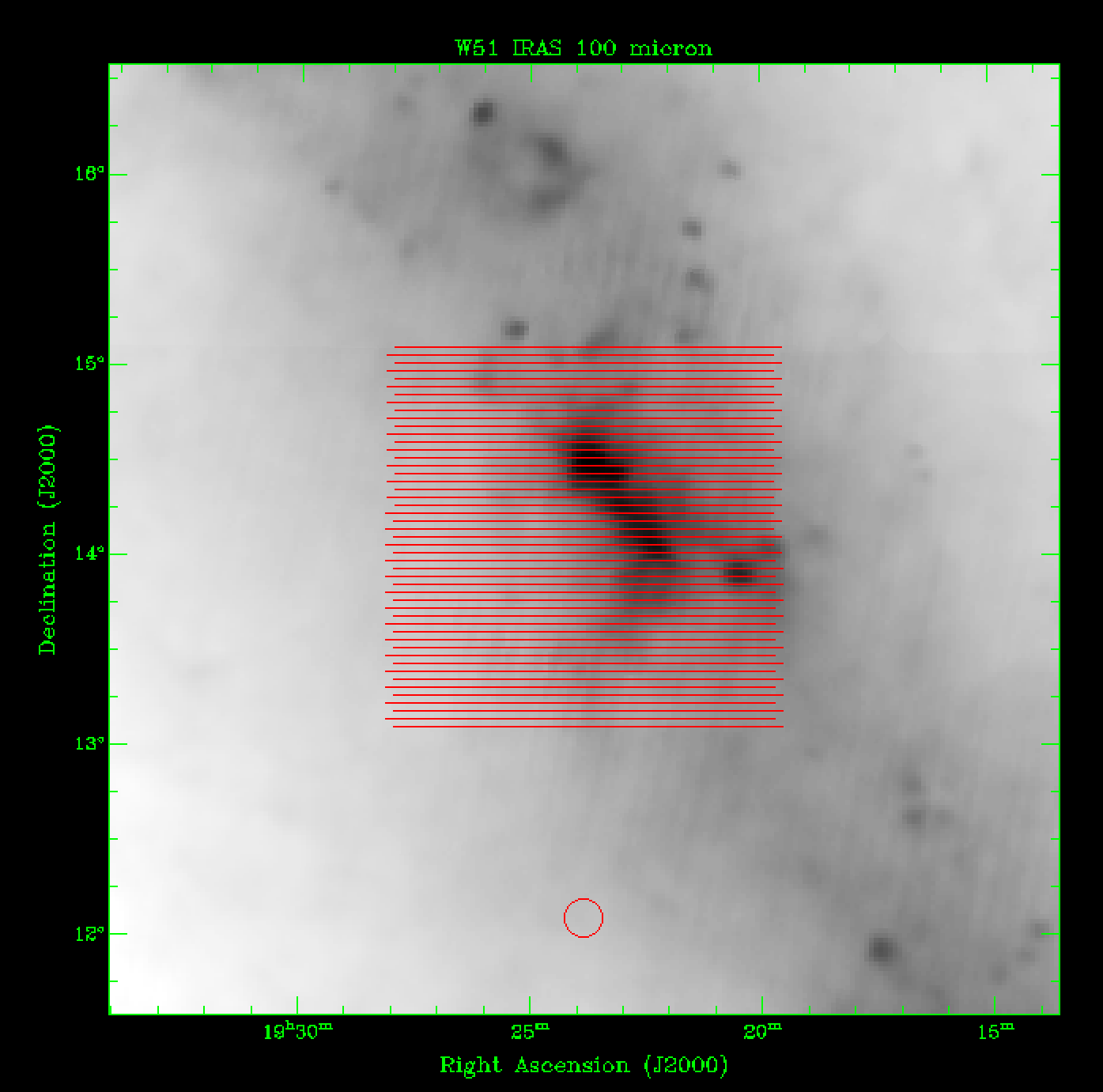
In this example, we show a Parameter Set for an on-the-fly (OTF) map of the HII region, W51, with selected subbands the same as in the previous example. We will create a 2 degree map of the region done with RA scans (scanning in lines of constant Declination), with a reference position located away from the HII region, which will provide bandpass calibration. We will revisit the referenced position after 5 scans are completed. Whilst orthogonal scanning is possible (i.e., RA and Declination), only RA scans are shown in this example, but you should aim to "basket weave" your maps (perform orthogonal RA and Declination scans) to gain better signal-to-noise, plus remove possible stripping when gridding. If you perform mapping in one direction only, you can oversample the row spacing between scans to account for stripping.
Tip
Due to the timing between the antenna starting a scan and Medusa starting recording, to ensure the start and end positions are recorded in the scan, pad the map width by 2xFWHM of the smallest beam being used. For example, in the above example, subband 20 has a beam FWHM 8 arcmin; add 2x8 = 16 arcmin to your map width.
The Nyquist row sampling for our RA scans should not be larger than (Equations 8,9; Mangum 2007), where D is the antenna aperture at the observing wavelength. However, depending on your region size and time constraints, it is perfectly acceptable to oversample the row spacing as mentioned above. For each scan, the 2 degree length will be done in 2 minutes, equating to a scanning rate of 1 degree/min. At this rate, beam smearing is not a factor when scanning away from Zenith (~ 10 degrees), or the South Celestial Pole, where parallactification can produce poor baselines; W51 is to the North and low on the horizon, so these effects are not in consideration anyway. In general, scanning rates should not be more than 3 degrees/min. For this example, we should note the beam FWHM is different for each subband as shown in Figure 2.10, with subband5 (1408 MHz) having a FWHM 15 arcmin, and subband20 (3328 MHz) about 6 arcmin. In order to satisfy the Nyquist spacing condition, we use the smallest beam (subband20) to define our row spacing to be 2.5 arcmin using the equation above, but also note this will oversample the lower subband (subband5) by a factor 2.4.
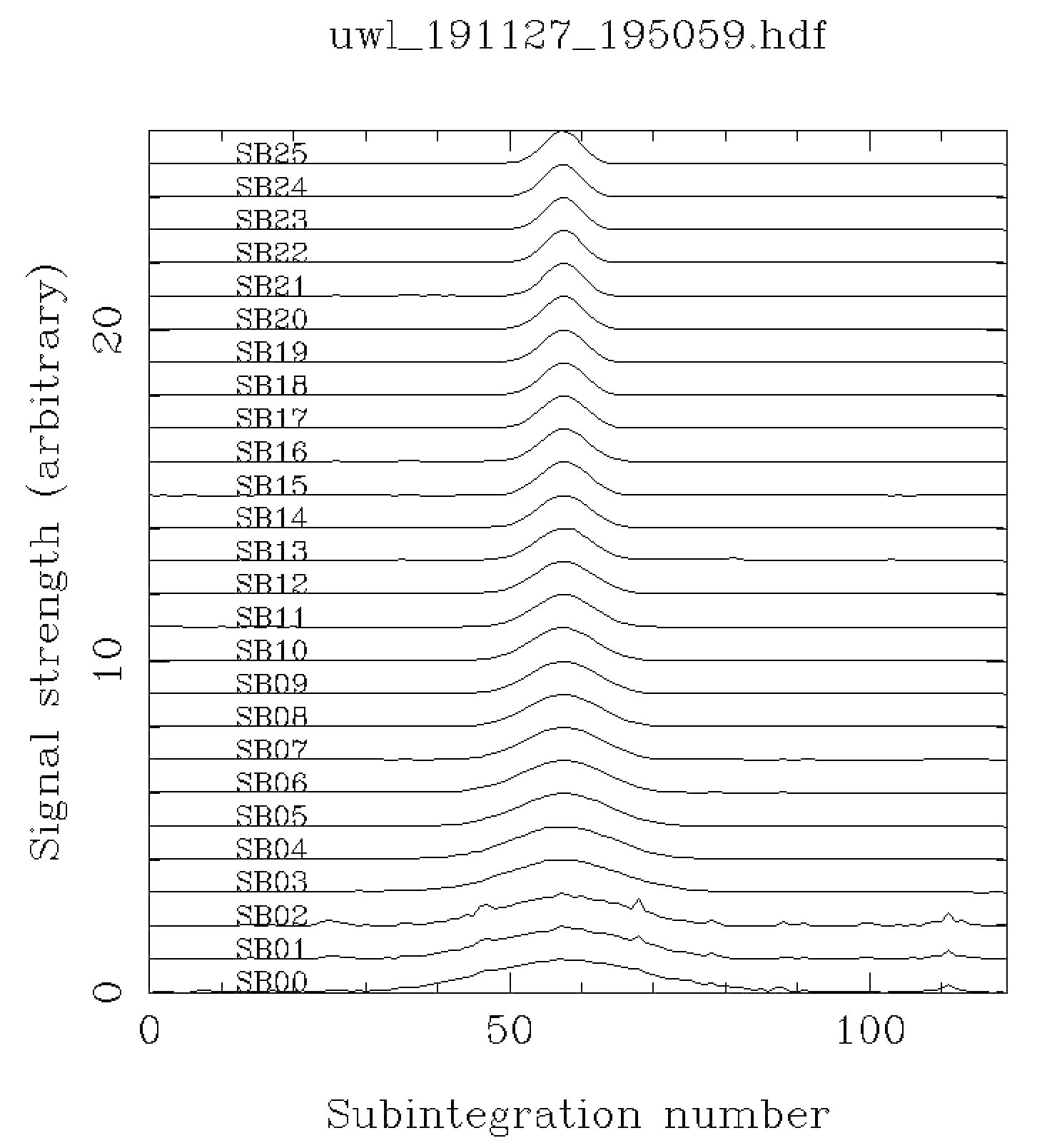
For each subband, MEDUSA will dump spectra every 5 seconds (output_tsamp) and the number of dumps per MEDUSA file is set by the sub interval time (output_tsubint) divided by the dump time (in the example this is 6, 30/5). To note the output_subint parameter is used for MEDUSA, but is not incorporated into the data file the observer receives from EURYALE. However, it is important to ensure that output_subint is an integer multiple of output_tsamp or MEDUSA will not record data. Using the determined Nyquist row spacing above, you can define a scanning rate using the following (in arcsec/sec), (Equation 10; Mangum 2007). For the example here, a 1-degree/min rate has the oversampling factor about 1. Having larger values for implies better signal-to-noise, but without frequent observations of the reference position between scans, drifts in the system (atmosphere, pointing and sky rotation) may mean your baseline subtraction may not be effective.
Now we input our parmeters into Dhagu?, as shown below. Under the "Editor" tab, select the ScanMapContinuum option from the select menu, and the configuration tool as shown below in Figure 2.11 appears. Here we are generating a square 2x2 degree map, using constant latitudinal (small-circle) scans and no rotation. Once the parmeters are entered, click on Generate and the Editor table will auto-populate with both tracked reference and scanning positions.
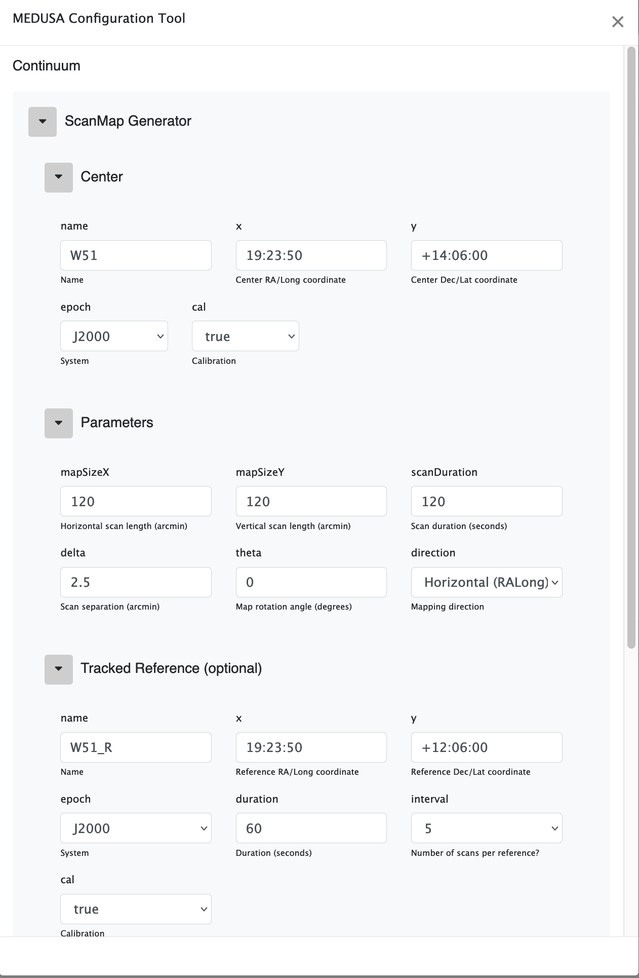
The result is 59 entries, with 10 of those the referenced track positions. Configuring MEDUSA is the same as per other examples above, and is left as an exercise.
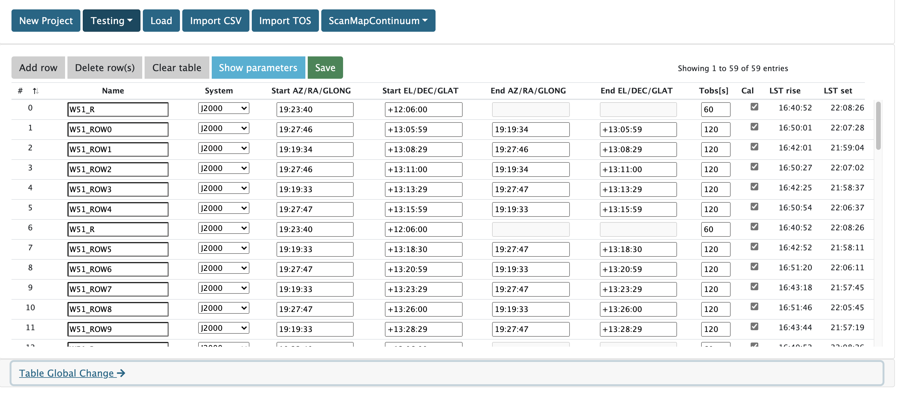
By clicking on the Show parmeters button, the (abbreviated) Parameter Set is shown below.
        cal.duty_cycle = 50
	cal.frequency =	100
	cal.phase = 90
	common.target.src1.cal_signal =	true
	common.target.src1.duration = 120
	common.target.src1.end_direction = [19:19:34,+13:05:59,J2000]
	common.target.src1.field_comment = Strong CH emission
	common.target.src1.field_direction = [19:27:46,+13:05:59,J2000]
	common.target.src1.field_name =	W51_ROW0
        .
        .
        .
In a future release, it may be possible to display Parameter Sets of region(s) using a framework like Aladin. The example below shows the generated RA scans overlaid on a 5x5 degree IRAS 100 micron image using KVIS and the Dhagu?-generated annotation file. The reference position is shown as a circle to the South.
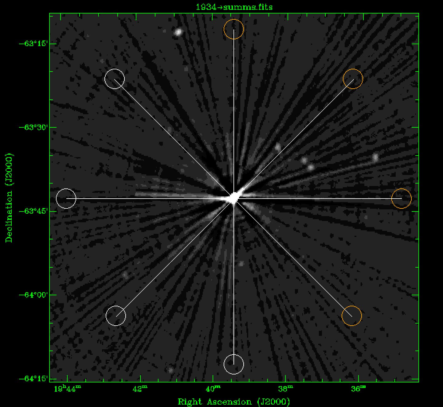
In this example, a Parameter Set for scans across the standard flux calibrator, PKS 1934-638 is outlined. By scanning across this source, we can determine the frequency-dependant beamshape and obtain the flux calibration. In this example, PKS 1934-638 will be scanned across in 1-degree strips, with scan angles 0, 45, 90 and 135 degrees. To ensure the source lies at the center of the scan, the scan mode will be set to a great-circle scan for the 0, 45 and 135 degrees scans, and small for the 90-degree scan (as lat1 === lat2). Note positive angles correspond to a clockwise rotation, with North = 0 degrees. A 0-degree angle with positive scan length corresponds to a scan in the North-South direction.
There is no MEDUSA configuration associated with this Scan example; this may be useful if MEDUSA is to be configured manually. By selecting Scan mode, we see a popup asking what calibration waveform configuration we wish to define. By clicking on the Save button, scans can be added as show in Figure 2.14.
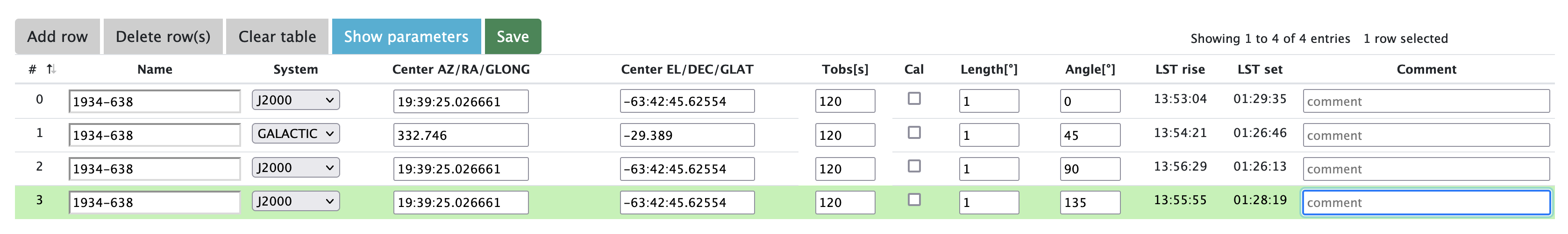
The orientation of the scans about PKS 1934-638 is shown in Figure 2.15. The pixel data is from the SUMMS 843 MHz Survey. The green circles determine the start of the scan. We can reverse the direction of the scan by defining the length as a negative number. In this situation, the starting position of the scan is identified by the white circles. If you wanted to do a scan across a source in an East->West direction and then the (reverse) scan from West->East, you would simply define the East->West with a positive length, and West->East as negative.
In this section, we setup the system to observe the pulsar J0835-4510 in fold mode using the MARS receiver. First, we ensure the receiver is turned on and on-focus as descriibed in Section 3.1.4.1.
Now under the Editor tab in Dhagu?, we select the TrackFold option from the Template select... dropdown. Under the Common menu, change the receiver to MARS. This will present additional options for enabling the legacy conversion system and switch matrix; set these to true. The configuration for Common will look as below.
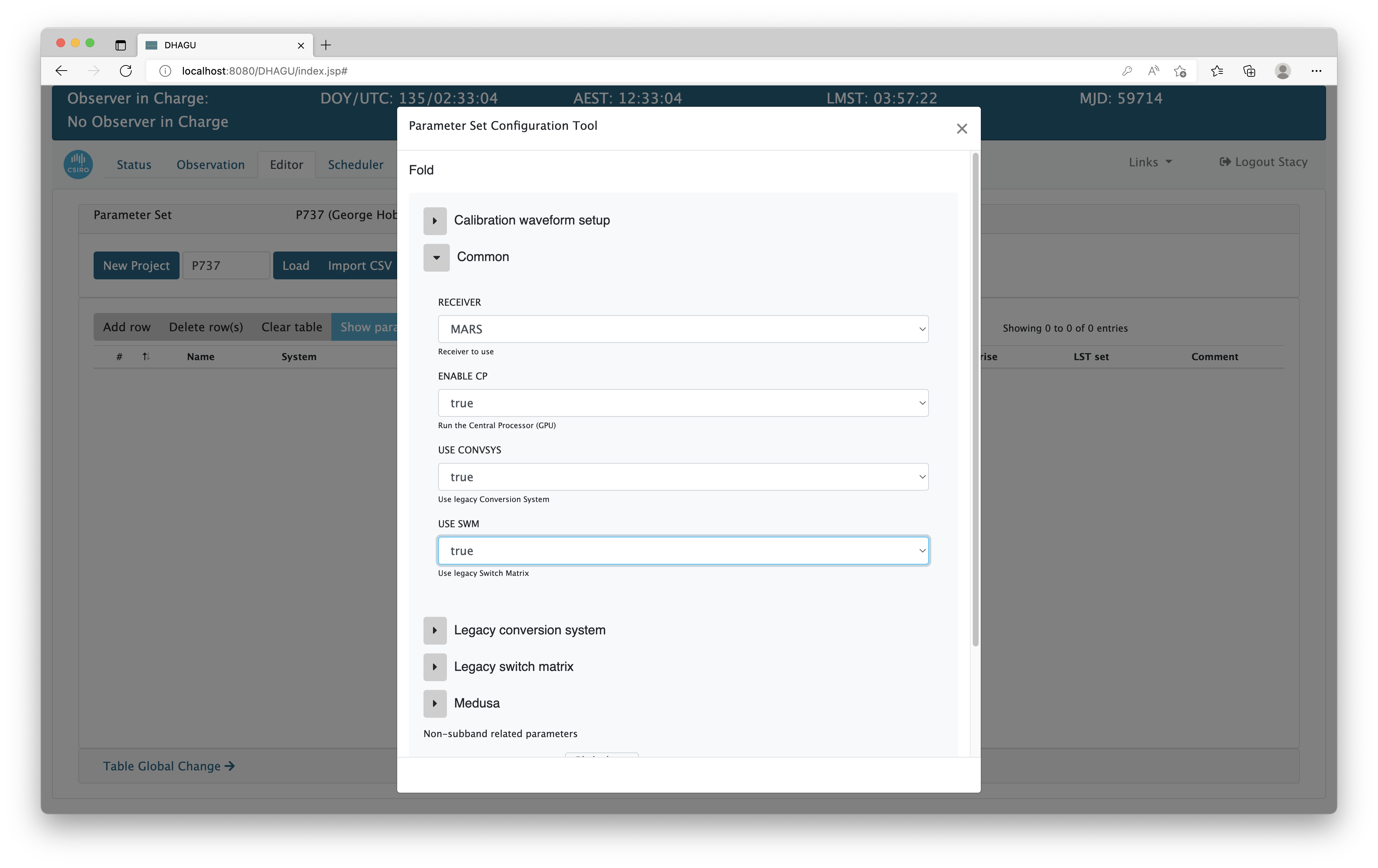
Next, expand the Legacy conversion system and Legacy switch matrix options. You will need to input the require conversion system lorun script TOS should run, see Table 2.2 for current options; we use mars_8457.cmd, which has centre sky frequency of 8457 MHz. Typically, you don't change the settings under Legacy switch matrix, so unless directed otherwise, leave as set.
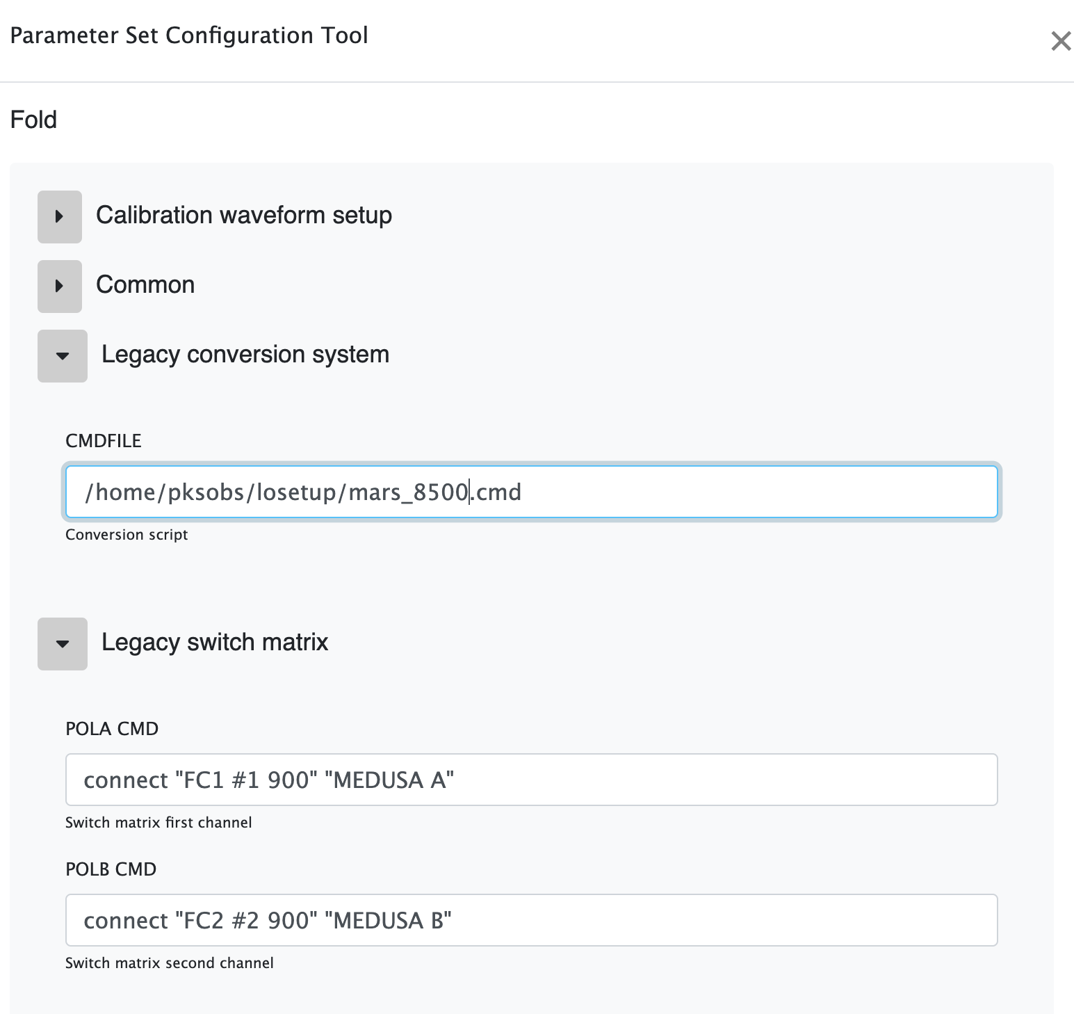
For the Medusa configuration, expand Medusa -> Common. Under this menu, you need to change the FCM CONFIGURATION to apollo.mars, plus change SUBBANDS to 8. Next, we want to configure all subbands with the same settings, so expand the Global option, select all subbands and configure as shown below. You can see the centre frequencies of each subband (note the reversed order indicating an inverted down conversion.)

Once the desired Medusa configuration is done, click the Save button.
Caution
Once you have saved a parameter set, you cannot change the receiver. If you need to change, click the Clear button at the bottom of the Parameter Set Configuration Tool, but note this clears the entire Medusa configuration.
Enter the positions for the calibration and on-source positions of J0835-4510 as usual. The final Parameter Set and observed frequency verses phase plot is shown below.
	cal.duty_cycle				= 50
	cal.frequency				= 11.1231
	cal.phase				= 90
	common.enable_cp			= true
	common.receiver				= MARS
	common.target.src1.cal_signal		= true
	common.target.src1.duration		= 120
	common.target.src1.field_comment	=
	common.target.src1.field_direction	= [08:35:20.6,-45:00:00,J2000]
	common.target.src1.field_name		= J0835-4510_R
	common.target.src1.obs_type		= TRACK
	common.target.src2.cal_signal		= false
	common.target.src2.duration		= 3600
	common.target.src2.field_comment	=
	common.target.src2.field_direction	= [08:35:20.6,-45:10:34.8,J2000]
	common.target.src2.field_name		= J0835-4510
	common.target.src2.obs_type		= TRACK
	common.targets				= [src1,src2]
	common.use_convsys			= true
	common.use_swm				= true
	convsys.cmdfile				= /home/pksobs/losetup/mars_8457.cmd
	apollo.common.cal.tsys_avg_time		= 5
	apollo.common.cal.tsys_freq_res		= 1
	apollo.common.fcm_configuration		= apollo.mars
	apollo.common.subband%d.adaptive_filter_epsilon	= 0.1
	apollo.common.subband%d.adaptive_filter_nchan	= 1024
	apollo.common.subband%d.adaptive_filter_nsample	= 1024
	apollo.common.subband%d.enable_adaptive_filter	= false
	apollo.common.subbands			= 8
	apollo.fold.append_output		= true
	apollo.fold.custom_period		= -1
	apollo.fold.output_nbin			= 1024
	apollo.fold.output_stokes	 	= 3
	apollo.fold.output_tsubint		= 30
	apollo.fold.subband%d.active		= true
	apollo.fold.subband%d.custom_dm		= -1
	apollo.fold.subband%d.enable_sk		= false
	apollo.fold.subband%d.output_nchan	= 128
	apollo.fold.subband%d.sk_nsamps		= 1024
	apollo.fold.subband%d.sk_threshold	= 3
	swm.pola_cmd				= connect "FC1 #1 900" "MEDUSA A"
	swm.polb_cmd				= connect "FC2 #2 900" "MEDUSA B"
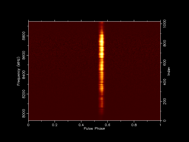
In order to become a qualified remote observer, you must complete the remote observer training. This is undertaken with a CASS staff member, via a Skype session, and typically takes about two hours to complete. The purpose of this training is not to instruct you on how to do an observation, but rather to acquaint you with the procedures and protocols of remote observing. Only people who have completed this training can carry out observations with Murriyang.
All observers will need a CASS Unix account and password. If you do not have one already, then you will need to organise an account and password before the training session begins. An application for a CASS Unix account can be made online, here.
It usually takes a week for the request to go through the system, so you should apply as soon as possible. Once the account has been organised, then you should request remote observer training by sending an email to: atnf-parkes-remobs[at]csiro.au. A date and time will be agreed on and the Skype addresses exchanged.
Following the training, you must then perform an observing session with a more experienced, qualified colleague, where you will be shown how to perform the specific observations related to your project.
Only when you have completed the remote observer training AND observed with an experienced colleague, will you be considered to be fully qualified.
All observing is considered to be remote observing since, regardless of where you observe from, whether you’re in the Murriyang control room or on the other side of the world, the same software is used.
To perform remote observing, you need three essential tools – the PORTAL which allows you to communicate with online staff and other observers; the FROG which provides you with situational awareness of the telescope through audio and visual feedback; and two VNCs in which the observing software is run and the various observing backends are controlled. NOTE: A fourth tool is now also available that allows observing to be conducted, with the UWL receiver, via a browser based system - Dhagu?, Section 3.1.2.7.
Ideally, we recommend that three separate screens be used to allow easy visual monitoring of the observation. In one screen we display the first VNC in which the observing software is run. On another screen we have the second VNC in which we run the correlator and other related software. Finally, in the third screen we have the PORTAL and FROG running in browsers. Since these two provide audio feedback, they should operate on machines that have a sound card with the volume turned up.
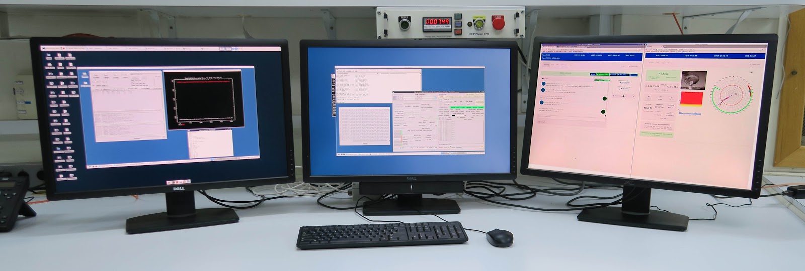
Figure 3.1. A typical setup for remote observing. L-R: Screen 1 with VNC2 running the correlator software; Screen 2 with VNC1 running the primary observing software; Screen 3 with the PORTAL and FROG. NOTE: This three screen setup is not essential, but it does allow for easy visual monitoring of the observation. Also to note for UWL observations, the first screen would be replaced with an additional web browser window containing Dhagu? and the second would show the VNC1 desktop but with the UWL GUI for LNA control and OPERFCC for receiver translation.
In order to begin observing, you will need a CSIRO Unix account and password. If you do not have one, then please arrange to obtain one at least 2 weeks before you begin the observing session.
In a browser, login to the remote observing PORTAL (for communications, details in Section 3.1.2.4), here.
and open FROG (for telescope monitoring, details in Section 3.1.2.5), here.
And open Dhagu? (for telescope control with TOS, details in Section 3.1.2.7).
It is important to ensure that you have audio enabled.
If you are taking over as the designated observer, firstly, alert the current observer to begin the hand-over process by typing a message in the chat window of the PORTAL. Then click on the Observer-in-Charge button and register; further details below.
In order to provide SSH access to ATNF facilities, please note there is now a change (as of 1st July 2025) required to improve security and better align with CSIRO IT and Australian Government requirements. The change applies only to connections from "outside" of CSIRO, to our SSH gateway hosts, "venice" and "orion". It will not apply to users connecting via CSIRO VPN with their CSIRO laptop, or to users connecting from "internal" networks. Instead of allowing login to venice or orion with a password or an SSH key, we will require users to use both a password and an SSH key. This is a form of two-factor authentication, which is being required across all of the Australian Government, including CSIRO. For more details, please visit here and here.
If you are observing from a non-ATNF site, you will need to tunnel into the ATNF network. Open an xterm on your local computer and type:
For joffrey:1
ssh -NfL 5901:joffrey.atnf.csiro.au:5901 ident@orion.atnf.csiro.au
In another xterm, type the following for joffrey:2
ssh -NfL 5902:joffrey.atnf.csiro.au:5902 ident@orion.atnf.csiro.au
If you want to monitor directly, via the SPIP page:
ssh -NfL 8000:medusa-srv0.atnf.csiro.au:8081 ident@orion.atnf.csiro.au
or, if on the internal CSIRO network:
https://medusa-srv0.atnf.csiro.au:8081/medusa/uwl/
NOTE: ident is your CASS Unix account (NOT your NEXUS account). If you have trouble accessing orion.atnf.csiro.au, you can also try venice.atnf.csiro.au.
Start the VNC client on your local computer and connect to 127.0.0.1:5901, which is the VNC1 window.
Start another VNC client on your local computer and connect to 127.0.0.1:5902, which is the VNC2 window.
To access MEDUSA, point your web browser to https://localhost:8000/medusa/uwl/ NOTE: If you see an error stating the connection is not secure, it is because the security certicifcate is only valid for addresses *.atnf.csiro.au and not localhost. It is left to the observer to determine the risks associated with continuing on or not. If in doubt, contact your IT department. Also, the SPIP page does NOT automatically load current status automatically. To do this, simply click on the required tab (TIMING, SEARCH or CONTINUUM) at the top of the SPIP page..
Note you can combine the above SSH commands into one as follows (as a single line):
          ssh -NfL 5901:joffrey.atnf.csiro.au:5901
              -NfL 5902:joffrey.atnf.csiro.au:5902
              -NfL 8000:medusa-srv0.atnf.csiro.au:8081 ident@orion.atnf.csiro.au
Or add the following to your ~/.ssh/config:
          Host orion
          HostName orion.atnf.csiro.au
          User ident
          LocalForward 5901 joffrey.atnf.csiro.au:5901
          LocalForward 5902 joffrey.atnf.csiro.au:5902
          LocalForward 8000 medusa-srv0.atnf.csiro.au:8081
Replace 'ident' above with your CASS Unix login ident.
You will need to login with the VNC password. This password will change at the beginning of every observing semester, so be sure to get the new password if you are observing for the first time in a semester. Visit this site for instructions on how to get the new password here. When observing from within CSIRO (either from an onsite computer or through a VPN), open an xterm on the computer you are using for the remote observing and start the vncviewers for joffrey.
For VNC:1, open an xterm and type;
vncviewer joffrey:1
For VNC:2, open another xterm and type;
vncviewer joffrey:2
The PORTAL allows the observer to communicate with other observers, to hand-over observing from one observer to the next, to troubleshoot, book observing sessions and generally setup and register as the current observer. It also allows the observer to post fault reports and find information and observing documentation.
The PORTAL can be accessed via a browser from this web address. Be sure to bookmark the address so that you can access it with ease, at a later time.
You will need a CASS Unix account and password to access the PORTAL. NOTE: Your CASS account is unique to you and it allows us to identify you and to determine if you are qualified to observe or not.
When an observer logs in, the alerts are first displayed in a message window. Alerts are issues that may cause problems during an observation. It is important to read these alerts every time you log into the PORTAL, since they are updated frequently. Take note of the alerts, and follow the instructions (if any) on how to avoid or mitigate the problems or issues. Once they have been read, click outside the alerts window to continue to the PORTAL’s main page. If the alerts were missed, then they can be accessed again by clicking on the Show Alerts button.
Alerts that are for your information only, are displayed in blue. Warning alerts, such as impending severe weather and RFI, are displayed in orange, and critical alerts, which will cause you to lose observing time, will be displayed in red. Note that for critical alerts, they are also emailed to any observers that have booked on the PORTAL. To cater for weekends, any critical alerts posted on a Friday are sent to all observers booked within the next 72 hours, or 48 hours if the issue occurs on a Saturday. The default is four hours, which is the same time use for weather-based (warning) alerts.
Once logged in, the times are displayed at the top of the PORTAL. The observing schedule is in Australian Eastern Standard Time (AEST), which is UTC+10 hours. It is important to note the time difference between AEST and the observer’s local time, so that a start time or finish is not missed - you don't want to be late for an observing session and lose that time.
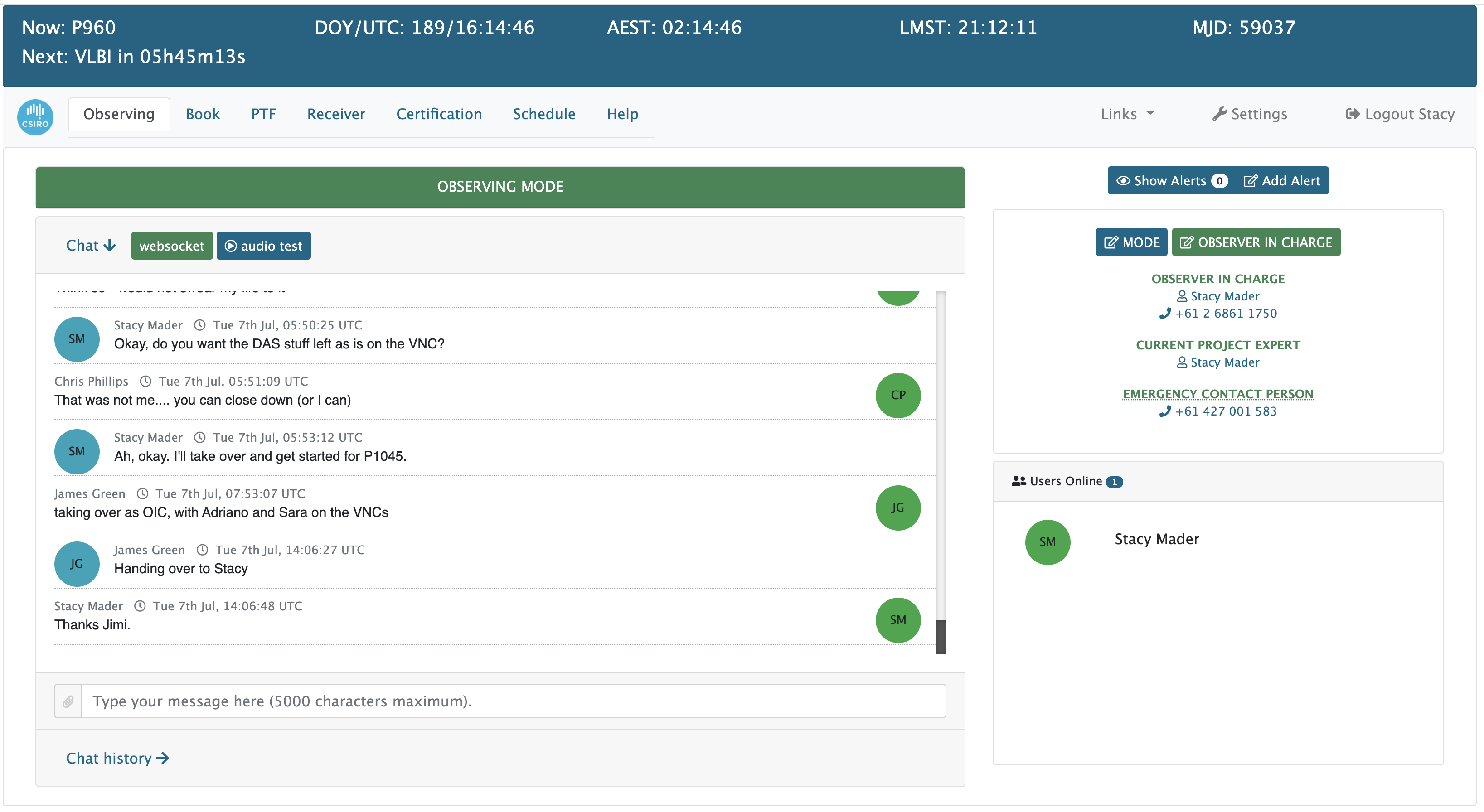
Modes of operation:
There are three modes of telescope operation – Observing Mode, Verification Mode and Maintenance Mode.
When the telescope is in observing mode, the mode is displayed in green with a green background and normal observations can proceed. The VNCs will be enabled and the observer can register as the Observer-in-Charge (OiC).
When the telescope is in maintenance or verification mode, the mode is displayed in red with a red background. The VNCs are disabled from outside access. Verification mode is intended for use by science operations staff to conduct post maintenance tests prior to hand over to observing. To note, you can't register as the OiC while in either of these modes. These precautions are necessary to prevent any off-site observer from inadvertently accessing the VNCs and taking control of the telescope and moving it about when maintenance is being undertaken. Staff may be on the dish surface, in the focus cabin, or elsewhere on the telescope. Moving the dish, or any other equipment, while work is being done on them could cause the staff members to be seriously injured or the telescope and equipment damaged. Only when the staff member who is responsible for the maintenance is satisfied that it is safe to resume observing, is the operating mode switched back to Observing Mode and normal observing resumed.
NOTE: Sometimes the maintenance runs overtime, or finishes earlier than planned. It is important to check the chat utility for notifications on when the observing will resume, to avoid missing an early start or arriving un-necessarily early if maintenance runs overtime.
Chat Utility:
On the left, is the Chat Utility. An observer types a message in the text box at the bottom and the message is then displayed in the box above it. The observer’s name, with the date and time that the message was posted, is displayed so that other observers know who they are communicating with. The OiC’s initials are displayed in green circles, while all other users are in blue circles.
Registering as the Observer-in-Charge (OiC):
It is important to register as the OiC as soon as possible after you take over. If there is no OiC registered, then the observing team is alerted via email and asked to immediately arrange an observer to register and do the observation. This is a security issue, since we don't want the telescope to be unattended and capable of being moved about with nobody in charge. There must always be someone in charge and looking after the observations. It also means that we can check that the person who has registered as the OiC, has undergone the Remote Observer Training and is certified as a qualified observer.
To register as the OiC, click on the Observer in Charge button. You will be presented with a pop up window in which you have to enter your contact telephone number. Select from one of the options in the pull down window. The contact telephone number for that location will be displayed, except for the “Other” option. If you are observing from a location that is not listed, select “other” and enter the telephone number manually. Be sure to include the country code and area code along with the telephone number. For example, +61268611755 is the number for the Control Room (+61 is the Australian country code, 2 is the area code, and the 68611755 is the control room telephone number).
Your name will then be displayed under the OBSERVER IN CHARGE (OIC) heading on the RHS. For privacy reasons, the telephone number displayed (+61 2 6861 1750), is a re-direct number to the telephone number you entered when you registered as the OIC.
If the observer is not certified, operations staff will be notified and appropriate action taken. The observer’s CASS Unix username uniquely identifies the observer.
Every day, a local staff member is rostered on to be the Emergency Contact Person (ECP) in case anything should go wrong with the telescope. For privacy reasons, only the mobile phone number of the ECP is displayed on the PORTAL. NOTE: The ECP should only be contacted if a serious issue arises and threatens the safety of the telescope. For all other issues, the Section 1.10.1 should be contacted.
The booking tab is where the observing schedule for the current semester is presented and where observers can book their observing sessions.
By default, the next seven days of the schedule is displayed when you first open this tab. Clicking on the “left” and “right” arrows on the top left hand side of the schedule, allows you to move forward and back through the schedule. It is also possible to change the view to fortnight, week or day.
The scheduled time is shown as coloured blocks.
- Grey: these are observing times that have not yet been booked by any observers.
- Light Turquoise: these are the maintenance times. Observers can not book to observe in these times.
- Dark Turquoise: these are observing times that have already been booked.
- Yellow: these are reconfigs when receivers are either installed or removed from the focus cabin.
- Green represents observing time that has not been assigned to any project. Observers can request to use this time as outlined below.
The times default to your local time, but this can be changed by clicking on the Timezone button. This makes it easier for you to schedule your observations to match your individual work schedules. NOTE: The local time is taken from the clock setting on your local computer or laptop.
To book an observation, move through the schedule to the date that you want to observe. For the relevant project block, put the cursor at the start time of your booking and drag the cursor to the end time. A popup menu will appear showing the start and end times you just selected. If these are not quite correct, click Cancel and retry. It is also possible to click any part of the block, then tick 'Snap to session start/end' on the popup modal. Note in either case, you are required to enter your email for contact purposes. You can also request a calendar file of the booking. After clicking Submit, your name appears for the range of times selected.
Observers can request Green Time by simply booking the Green Time as per the normal booking procedure above. Your request will then be emailed to the scheduler for approval, see Section 1.10.3.3.
It is important to book an observation because it allows the system to determine that a new observer needs to be trained beforehand. It also allows the PI to know that observers have signed up to perform the observations. Two weeks before the scheduled start of the observation, the system will check to see if anyone has booked the time. If not, the PI will be alerted by email that no observers have booked the time. The PI should then have sufficient time to organise experienced observers or to arrange new observers to be trained. The two weeks gives the PI enough time to organise the CASS Unix accounts and training, if required.
The Observing Expert tab contains a calendar which allows Observing Experts to assign themselves to observing sessions. It is possible to click and drag or batch book to register for projects. The resultant modal popup allows you to select or input an email address and phone number, then clicking on the "Register" button assigns you to that session. It is also possible to select an iCal file to be sent to the supplied email address.
It is possible to view current registered sessions using the "registered" button atop of the calendar. The modal popup shows all your registered projects. From here, you can also de-register from any selected observing session.
The PORTAL will send any registered Observing Experts a reminder one hour before the observing session starts. If there are no registered Observing Expert in the calendar but listed in the OPAL proposal, an email will be sent as a reminder to those Observing Experts to register for observing sessions. Note in the case where there are no registered Observing Experts in the calrndar, or available from OPAL, the last registered Observing Expert (within the last six months) for that project code will be assigned as the current Observing Expert for that session and sent an email notification.
FROG provides the observer with situational awareness of the telescope through audio and visual feedback. When the Murriyang version was developed, it was decided to give it a similar name to TOAD (Telescope Operator Alerting Display) which is in use at the Mopra observatory; since Mopra had TOAD, Murriyang was given a FROG.
FROG is a combination of some old observing tools, such as showtel and winds, plus a few new features that provide greater situational awareness for remote observers.
Like the PORTAL, the FROG can be accessed from a browser at the web address linked below. Also like the PORTAL, you will need a CASS Unix account and password to access it.
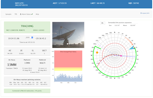
The Synoptic page on the FROG utility.
Left-Hand-Side: This is the region that shows you what the telescope is doing. It displays the coordinates of the position it is pointing at, what receivers are installed and which one is currently on the focus and being used.
Centre: A webcam image of the telescope is displayed here. It is updated every five seconds. It shows, in a single glance, the state of the telescope, that is, whether it is stowed or tipped over; whether it is day or night; whether it is clear or stormy etc.
Below this is the plot of the wind situation in the previous one hour. Every 20 seconds, the winds program looks back over the previous two minutes of wind data. It determines what the maximum wind speed was in that two minutes and also calculates the average wind speed in that two minutes, it then plots the data. The solid blue line is the maximum wind speed and the shaded blue region is the average wind speed. The coloured regions are:
White: As long as the winds stay in the white area of the plot, from 0 to 35 kph, then all is fine. However, with moderate winds and tracking low on the horizon and the wind coming from behind the antenna may still induce a low current stow.
Yellow: When the winds are in the yellow region, between 35 to 45 kph, then there is a high likelihood of the dish being wind parked at some point.
Orange: If the wind is in the orange region, between 45 to 50 kph, then you will very likely be wind parked.
Red: If the wind is in the red region, then it may be some time before you can resume the observations. You just have to wait for the winds to drop sufficiently for it to be safe enough to resume.
Right-Hand-Side: This is the sky plot visible from the site. The centre of the concentric circles is the zenith and the outer circle is the true horizon. They are in 10 degree increments. The red, inner circle is the telescope’s 30-degree elevation horizon. Your sources must be within this circle in order for them to be observable at the time.
The solid blue line extending from the centre to the edge, is the azimuth the telescope is pointing. The hollow red circle on this line is the position the telescope is pointing on the sky. The small solid, red circle is the position of the source on the sky and the red line extending to the left, is its future track, with the remaining tracking hours marked on it.
Behind the dish are two dashed, blue lines, creating a 60-degree segment (30 degrees either side of the back of the dish). It is important to avoid having the wind in this direction if the winds are high, since the wind will tend to push the dish down, creating a high likelihood of a wind park.
The blue arrow head jumping around the inner edge of the outer circle, is the wind direction. It grows in length as the winds pick up. When the arrow head reaches the centre of the circles (the zenith), the telescope will be wind parked. The cloud of orange dots around the arrow head are the average wind directions over the past hour. The darker the dots, then the more recent were the average wind directions.
The orange solid circle is the position of the Sun, and the grey solid circle, is the Moon. It’s good to know where these two are, in case you happen to be pointing at them and wondering why you can’t detect your source. FROG will issue an audio alert if you are within one degree of these objects.
Around the outer circle is a green curve with a cut-in. This is the wrap limit of the telescope (see Figure 1.10). The telescope cannot simply turn round and round forever, in azimuth. At some point it will need to stop and go around the other way. The two wrap limits are at the 205 degree and 295 degree azimuth positions. The active limit is shown as a cut-in. You cannot cross these limits. When slewing from one source to another, the control system will slew the telescope in the appropriate direction to avoid crossing the active limit. However, when it passes the crossover point at 68 degrees azimuth, the green curve will flip and the cut-in will be shown at the new active limit.
As the telescope slews from one source to the next, a yellow progress bar will appear on the outer edge of the horizon circle. The slew time and time remaining will also be displayed.
Just above the sky plot is a settings icon. Clicking on this will bring up a menu. You can select additional items to display such as the planets, the galactic plane and various satellite constellations. Certain satellite constellations could have transmissions in your observing band. By knowing where they are on the sky, you can better avoid them to minimise RFI. With the Solar scatter lobes option, you can display the scattering cones of the three feedlegs of the antenna. When a strong source (such as the Sun) lies within one of these scattering cones, radiation will be reflected off the feedlegs, and into the receiver. This option is useful to help minimise Solar ripple in data during daytime observing.
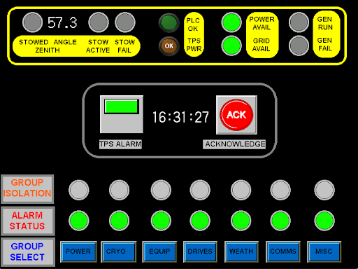
Figure 3.4. The TPS display in the control room. This can be accessed by the ECP to remotely resolve the issues and problems.
The Telescope Protection System (TPS), is a device that monitors hundreds of data points on the telescope. If it detects an issue that might be a major problem or concern, then the Emergency Contact Person (ECP) is alerted via SMS and various other alarms. The ECP can log into the system to see what the problem is and if needed can be at the telescope within minutes to resolve the issue and make the telescope safe. The TPS page on the FROG displays the various monitoring points. If one or more of these is red, the observer can see what the issue is by clicking on the link. A popdown menu will appear showing a summary of the issues. This display is only for information only. It cannot control the TPS. The ECP however, is able to log into the TPS to remotely resolve the issues and problems.
The TPS display in the control room. This can be accessed by the ECP to remotely resolve the issues and problems.
Note that Grafana may soon be replacing FROG. Currently, the Grafana instance is only accessible from within the CSIRO network and the FROG page can be accessed here.
For TOS/ observing, you will need to log into Dhagu?.
Whilst it is possible to login at any time to create Parameter Sets and manage Scheduling Blocks, you will need to register as the Observer in Charge via the PORTAL to submit Scheduling Blocks to the Observing Queue. The current Observer in Charge is displayed under the Observation tab in Dhagu? Note that when you register as Observer in Charge, you then have the ability to remove any Scheduling Blocks that are queued from the previous observing team.
Handover between observers is done via the PORTAL. Observers should login prior to the start of their allocated time and open a line of communication with the current observer. Ideally this is done at least 5 mins prior to the hand over and allows for the current observer to cleanly finish their observations. The expectation is that the current observer finishes in time to hand over at the allocated time unless an agreement has been made between the two sets of observers (for example if the current observer needs an additional few minutes to complete the current scan and the next observer is not time critical). If the current observer is unresponsive on the portal the new observer should allow a period of up to 5 minutes grace before taking over control. If there is no incoming observer ready to take control, the telescope should be stowed and the encumbent observer deregisters.
If the handover is between local staff from a maintenance session to remote observers then the same PORTAL process is followed, but is subject to the completion of any maintenance activities. This exchange will also involve the switching from ‘maintenance mode’ to ‘observing mode’, done by the observatory staff.
The current number one golden rule for changing receivers is to only do so when the telescope is either parked or stowed - this is to reduce stresses on the telescope infrastructure. Please use the FROG interface to determine when the Dish is parked or stowed.
When the antenna is parked/stowed, you can move your required receiver to the focal point. However, it may well be it is already on focus, so check the "On-focus" section in FROG. In the joffrey:1 VNC window, find the ‘OPERFCC’ GUI. Ensure that the required receiver (UWL/...) radio button is selected and then click on the yellow box “place selected receiver on axis”. Wait until all the “status” lights near the top are green (takes a couple of minutes).
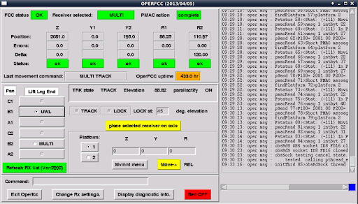
Once the receiver is on axis, you may need to power on the low noise amplifiers (LNAs); note that submitting a Scheduling Block with Dhagu? will automatically turn on the UWL LNAs, so VNC access is generally not required. However, the manual control for the UWL LNAs is (usually) located on the second screen in joffrey:1 VNC. The GUI is titled ‘CS-Studio GUI’. Select the ON button in order to turn all the LNAs on. If all of the LNAs don’t turn green, select the ON button again. Do not forget to turn off LNAs (via PKMC) for other receivers that are not on focus.
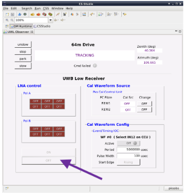
If you cannot find the GUI on any of the joffrey:1 VNC virtual desktops, you can restart the GUI by opening a terminal in joffrey and typing the following:
/usr/bin/CSS /usr/share/cs-studio/opi/parkes/uwb_obs.opi
You can also start the GUI from the "Observing Tools", "UWL Observer" menu item at the bottom of the VNC virtual desktop.
For the MARS and 13MM legacy receivers, you will need to use PKMC in the joffrey:1 VNC to switch the receiver package on, plus turn on the focus cabin synthesiser. The synthesiser is required to downconvert the signal into the S-BAND (MARS) or C-BAND (13MM) modules of the legacy conversion system.
To turn on the MARS and 13MM packages, click on the Other / Focus Cabin Switches / "show->" button. The GUI displayed should look as below. Typically, there willl be a "MARS Rx", or "13MM Rx" button which needs to be pressed such that the button turns from Off (red) to On (green). Note the "UWL Rx" button is always On (green). The next step is to switch on the focus cabin synthesiser, so press the "FC Synthesisers" button to switch it from Off (red) to On (green).
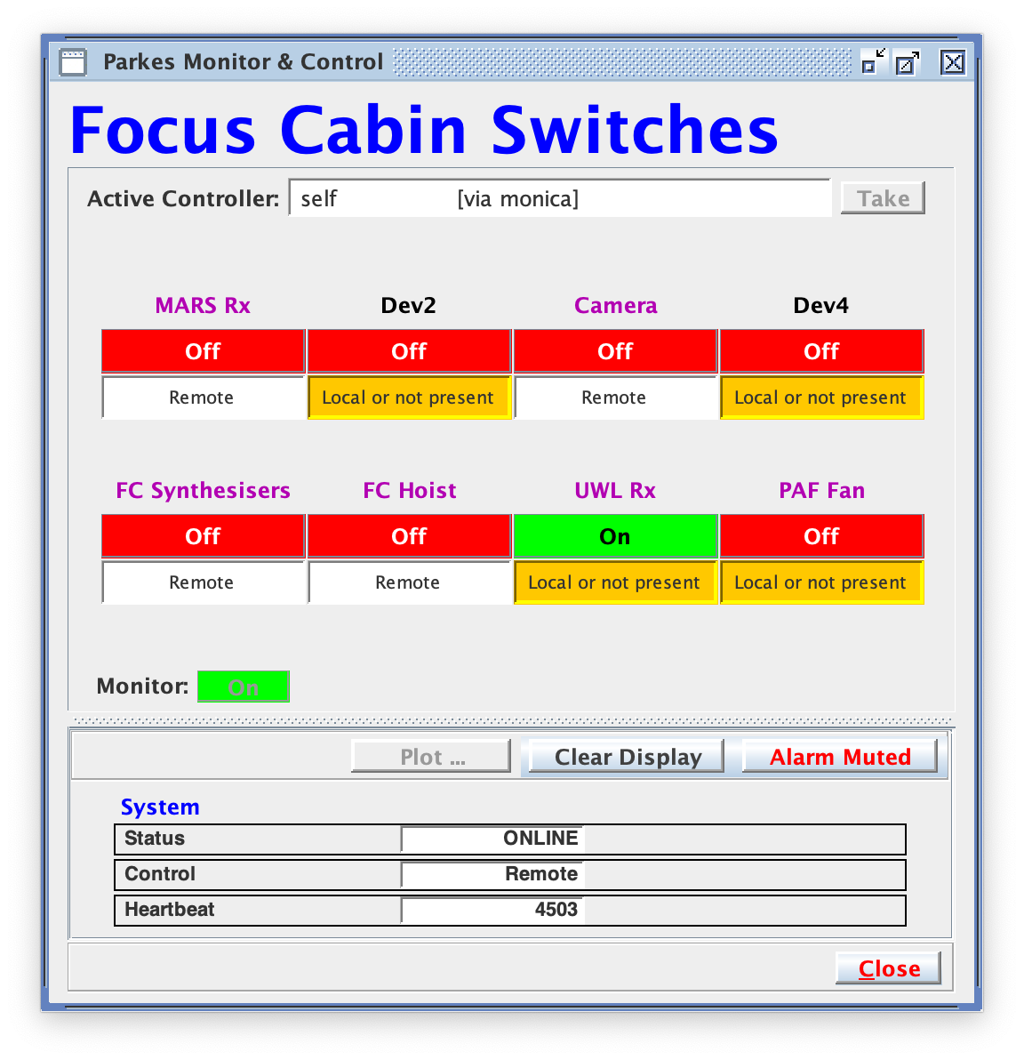
For the 13MM receiver, there is an additional step. Once you have powered the package and synthesisers to On, you will need to turn on the LNAs. On PKMC, click on the Receivers / 13 mm / "->show" button and the 13MM control GUI will display as below. Click on the "LNA A" and "LNA B" buttons to turn them to the "On" state (green).
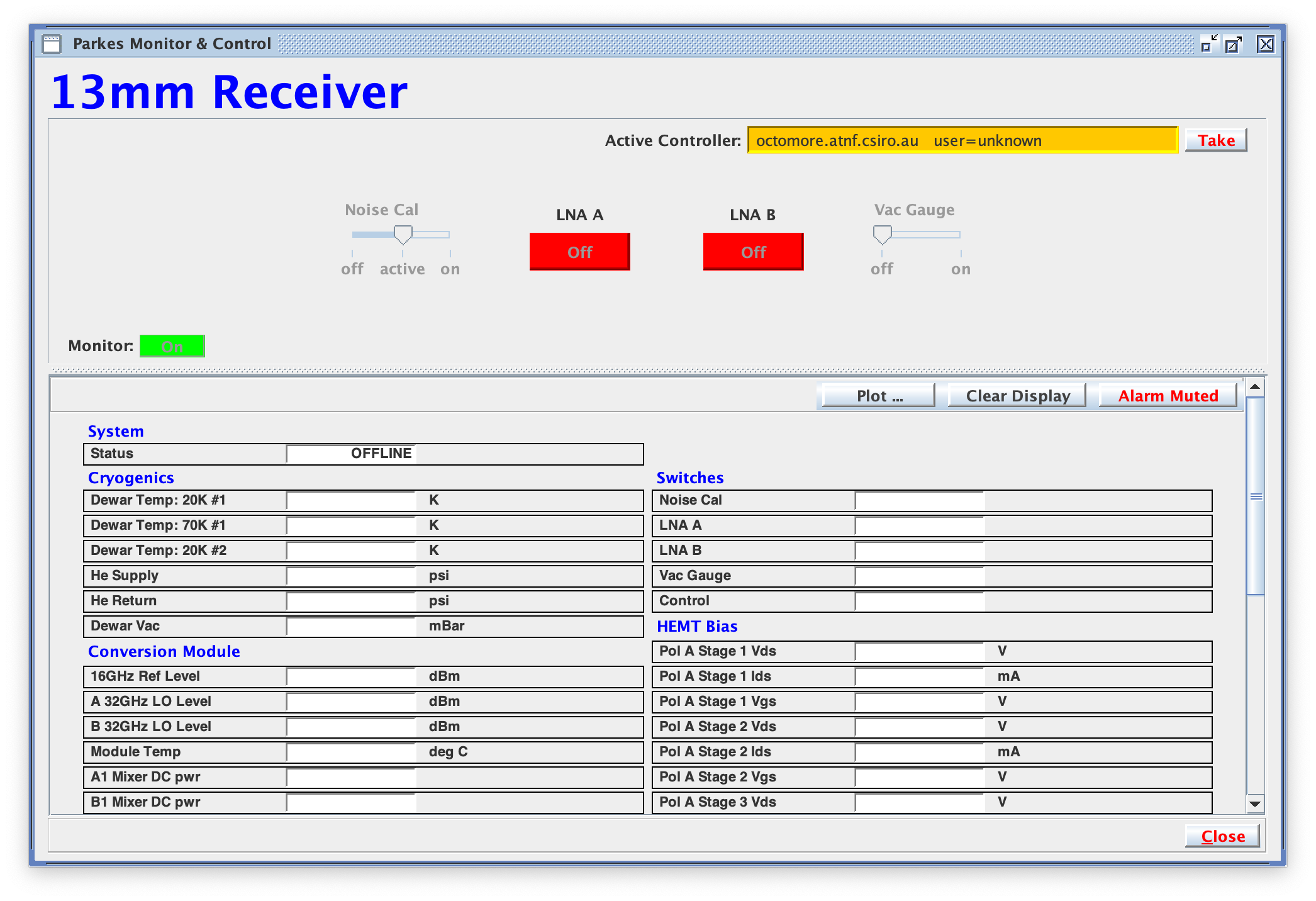
Caution
When your scheduled observing is completed, you should park the antenna and switch off the receiver package and focus cabin synthesiser. Failure to do so may cause interference for other projects using other receiver systems.
Dhagu? currently consists of multiple tabs, each designed to allow monitoring and submission of Scheduling Blocks. Each will be described below.
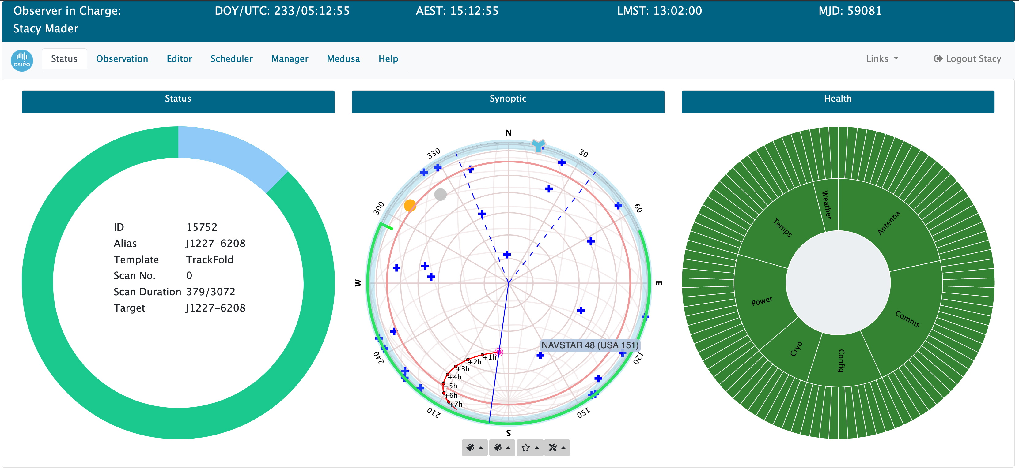
This tab gives the observer a general overview. The left panel shows the Status section, and the current state of the Observing Queue and current Observer in Charge. In the center panel, a a synoptic view of the antenna is shown, with options to display planets, the Galactic plane, plus particular satellite constellations, or those satellites that fall within particular subbands of the UWL system. The right panel shows health status for various TPS monitoring points. Clicking on a section will zoom in and clicking on the central circle allows you to zoom out. Presently, there are no monitoring points associated with the UWL receiver, or MEDUSA.
The circular donut is a graphical representation of the Observing Queue. When a Scheduling Block is running, information about the Scheduling Block is presented therein (Scheduling Block number, scan number, …). When the Observing Queue is running, the underlying donut should be green. When stopped or aborted, the donut will be red. When a Scheduling Block is running, the countdown will be shown as the blue overlay, incrementing until the Scheduling Block completes. The Observing Queue runs Scheduling Blocks in time mode, where the Scheduling Block ‘scheduler.time’ variable is used to determine the order, with the closest to the current time run first. There is a FIFO (First In, First Out) mode, but this mode is currently not in use.
The synoptic view is essentially the same as that in FROG. However, there are a few differences in that the display is an Orthographic projection, whereas FROG is a flipped Stereographic projection. Currently, satellites (whether a particular constellation, or within a subband), planets, flux calibration sources at different radio bands (LS, CX and K-band), and the Galactic Plane are options, available from the menus at the bottom of the display.
The Health indicator shows TPS monitoring points for various subsystems- Antenna, Comms, Config, Cryo, Power, Temps and Weather. Beneath these, are individual monitoring points. You can view these points by clicking on any top-level panel. To zoom out, click on the central circle. If any individual point is in an alarming state, it will turn from green (status = ONLINE), to red (status = OFFLINE). As a result, the parent panel, will also turn red, to indicate there is an issue. Presently, there are no audio alarms associated with an OFFLINE state. Also, there is no monitoring of the UWL receiver, or , but these will be added when available.
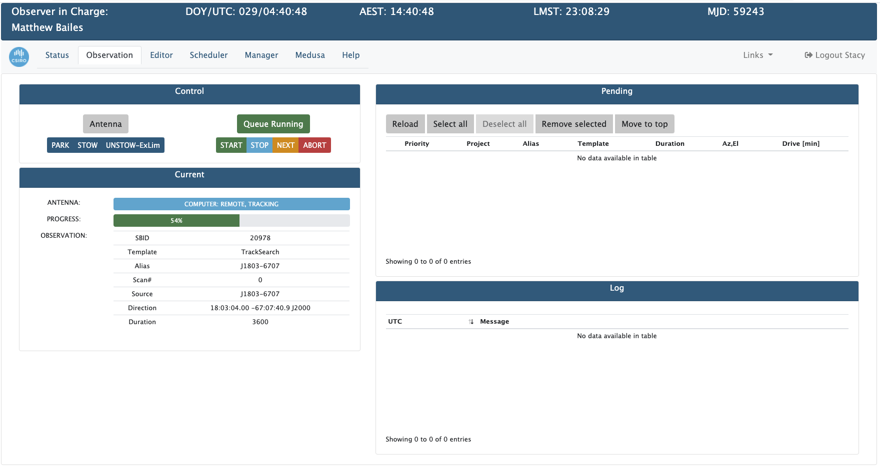
Under the Control tab, we see the ability to park, unstow and stow the antenna, plus Observing Queue controls. Note if the antenna is stowed, it will be automatically unstowed when a Scheduling Block is submitted to the Observing Queue. To access these controls, you must be the Observer in Charge, currently set via the Observing PORTAL. In order to park, unstow or stow the antenna, the Observing Queue must first be empty, that is, there must not be any sources in the Pending table to the right. If you attempt to initiate a park, unstow or stow with a non-empty Pending list, you will be prompted to remove sources prior to the park, unstow or stow being executed. The START, STOP, NEXT and ABORT buttons allow the observer to control the state of the Observing Queue. The START button initiates the Observing Queue, allowing Scheduling Blocks to be executed. The STOP button allows the observer to gracefullly exit the Observing Queue after completion of the current Scheduling Block. The NEXT button allows you to stop the observation in progress, and automatically start the next source in the Observing Queue, if any. The Scheduling Block will transition from EXECUTING to OBSERVED automatically, and this may be of use when your S/N ratio is sufficient and you want to continue on to the next source. The ABORT button stops the Observing Queue, and transitions any currently executing Scheduling Block from EXECUTING to ERRORED; you can transition this Scheduling Block to another state (OBSERVED, RETIRED) via the Manager tab.
Caution
Note the Observing Queue will stop if the antenna is wind parked. It is the responsibility of the observer to check weather conditions allow safe observing before re-enabling the queue.
This tab shows the current state of the antenna, progress as a percentage of total time complete, plus information on the currently executing Scheduling Block. This includes the Scheduling Block number, template, alias, source name, requiested position and duration.
This table shows sources currently available to be placed on the Observing Queue, and is populated by loading and selecting sources from a Parameter Set from the Scheduler tab. For each source listed, the priority (see below), project, alias, template, duration, current Az/El of the source and drive time are shown. In this context, the drive time (in minutes) represents the drive time for the antenna to a particular source from the current location of the antenna. Sources in the Pending table can be reordered by clicking on a row and dragging it to the desired position in the list. The priority here is such that the source at the top of the list will be the next source to be observed. Sources can be added anytime via the Scheduler, with the current behaviour being a new source will be added to the bottom of the current list. If you wish to move a source to the top of the list (single selection only), use the Move to top button, or use click+drag to place the source where required.
The Pending controller runs every five (5) seconds to see if all of the conditions below are met. If so, the next source in the Pending table is popped off the list and submitted to the Observing Queue.
- The Master Control Panel (MCP) must be in computer remote.
- The Observing Queue must be running (via the START button).
- A Scheduling Block must not be currently running.
The ability to reorder the Pending list is useful if you are (say) wind parked and only 50% of the Scheduling Block was completed. You can reschedule the same source from the Scheduler tab, and move to to the top of the Pending list and continue when the wind abates. Another benefit is your can reorder the list based on the drive time, to minimise slewing times. As in previous versions, there is no longer the need to remove other sources in the pending list if you wish to resubmit a source. You can also remove sources in the Pending list anytime by using the Remove selected button.
The log from TOS is displayed here. Along with the progress of the Scheduling Block, errors will be also presented. Messages are colour-coded, according to status, with red highlighting an ERROR, and normal messages in blue and warnings in yellow. The log associated with a Scheduling Block can also be viewed from the Manager tab.
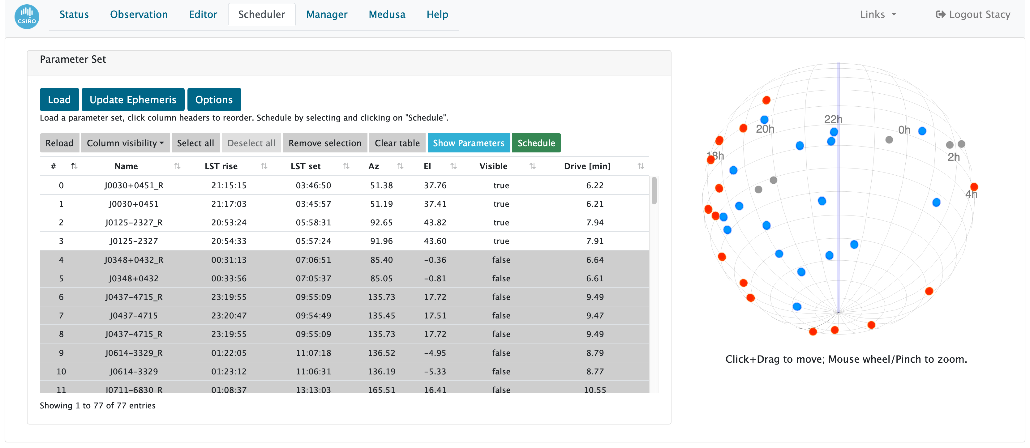
To load in a Parameter Set, click on the Load button, select your project and a list of all Parameter Sets will be displayed, as shown below.
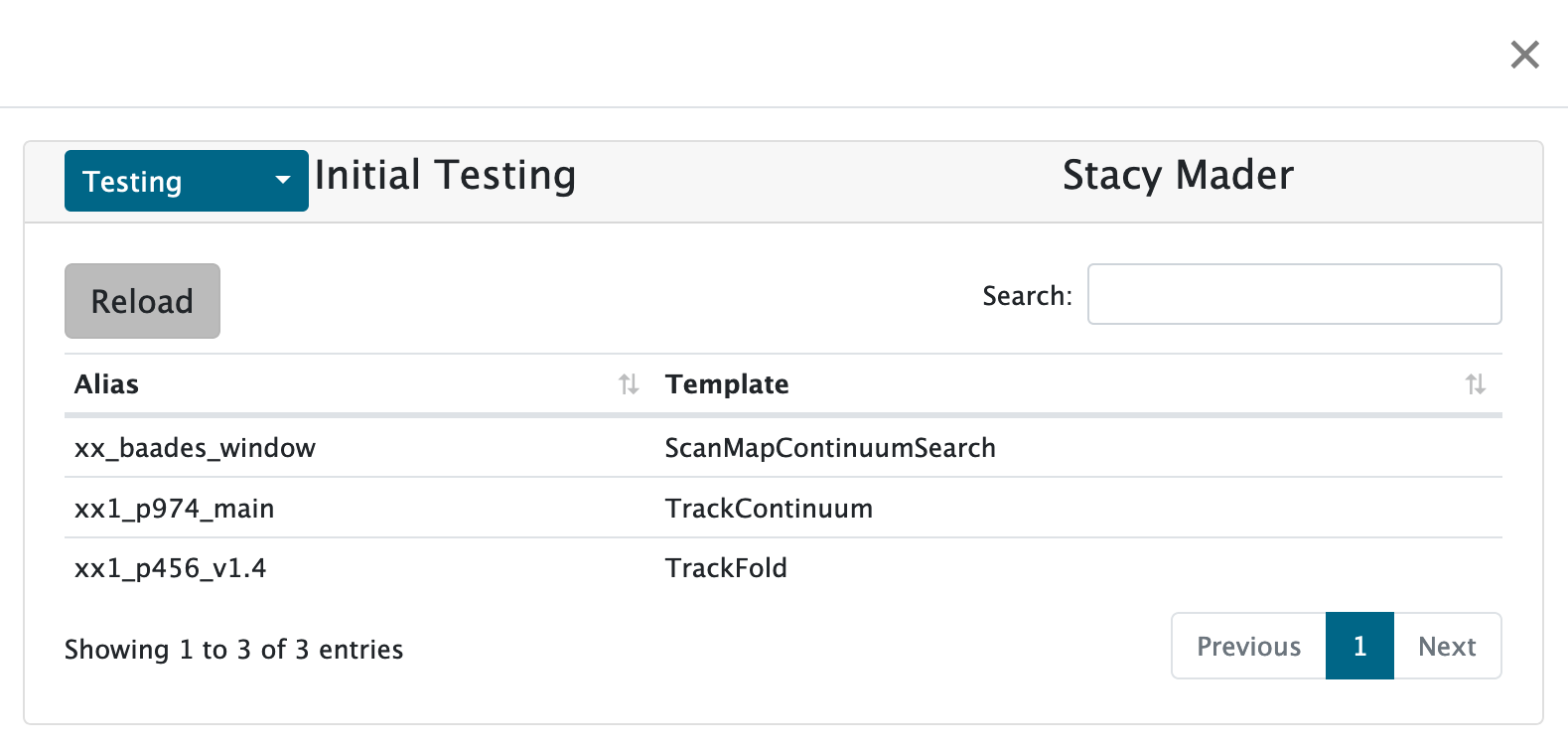
Click on the required Parameter Set to load. Once the Parameter Set is loaded in, you can view the Parameter Set by clicking on the Show Parameters button.
To submit sources to the Observing Queue, simply select sources, then press the Schedule button. Note the Scheduler table allows multiple column sorting, to help identify sources which are visible. Sources which are not yet above the horizon limit (30.25 degrees) are highlighted in grey. You can order the visibility column by clicking the ordering button next to the column title, and then, while holding the SHIFT key, click on another column ordering button such as Azimuth. This allows you to order the table by visibility (true/false) and increasing/decreasing Azimuth. To reset the ordering, simply click on the ordering button in another column.
Once sources are selected and the Schedule button is clicked, they will populate the Pending table, in the Observation tab.
A limited number of scheduling options are currently supported. These are accessible by clicking on the Options button.
- Auto refresh?: This will update the rise, set and visibility parameters of sources automatically, every 10 seconds.
- Hide Scheduled Sources: Selected sources are removed from the table when scheduled. You can click the Reload button to display all sources in the Parameter Set. Note that removing sources from the table is not propogated to other users using Dhagu?
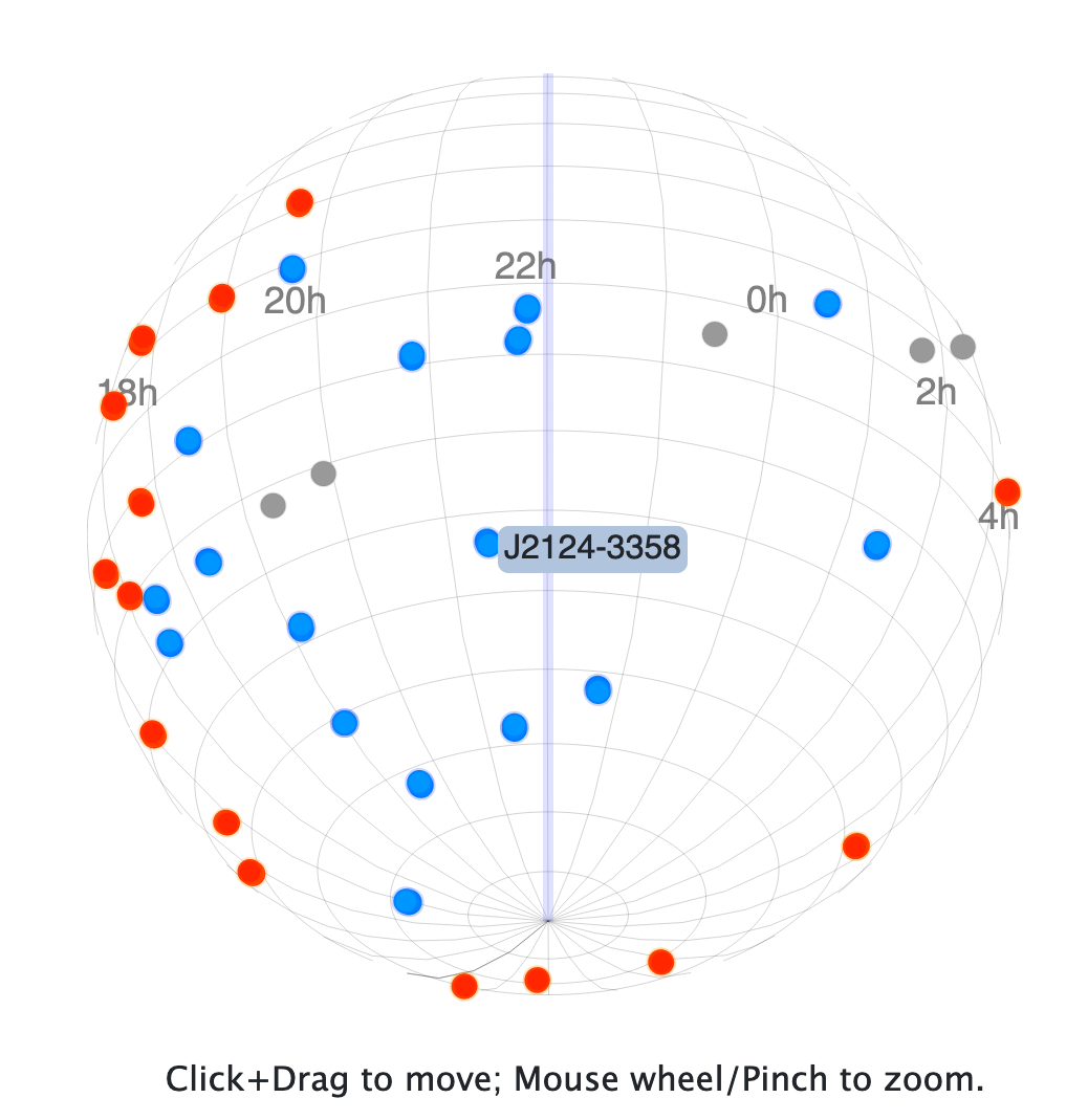
The position of sources in the loaded Parameter Set will be presented on the skyglobe in blue if currently visible (also check the table for visibility), and red if below the antenna horizon. You can click and drag the skyglobe to change the view. It is also possible to zoom in using pinch for mobile devices, or mousewheel; this is useful for crowded sources. The position of planets, Sun and Moon are also shown. The thin vertical line represents the current LST. You can press the Refresh ephemeris button to update both the positions on the skyglobe and Azimuth, Elevation, visibility and rise/set parameters on the table.
The Manager tab allows Parameter Sets for projects to be viewed, downloaded or retired. Scheduling Blocks can be transitioned to other states, plus submit comments or create a Jira ticket for any issues associated with the Scheduling Block.
By selecting a project from the dropdown menu under Available Parameter Sets, a list becomes visible. The observer can click on any to view key/value pairs, or download/retire the Parameter Set via buttons at the bottom of the popup. Note that retiring a Parameter set means it will no longer be visible or selectable from Dhagu?
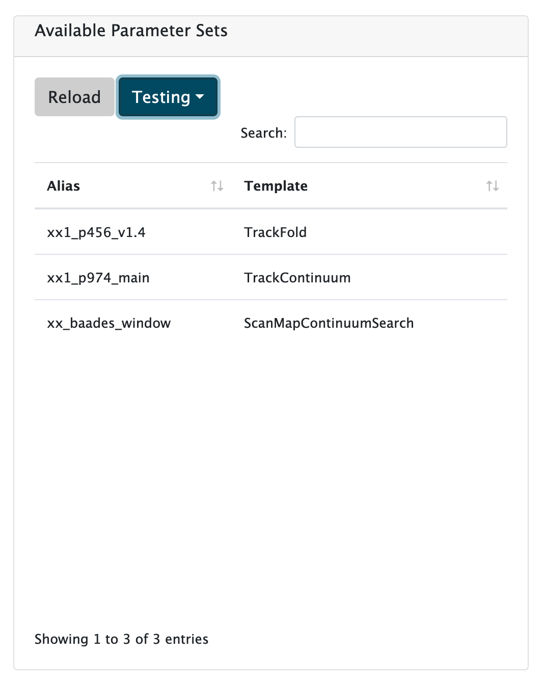
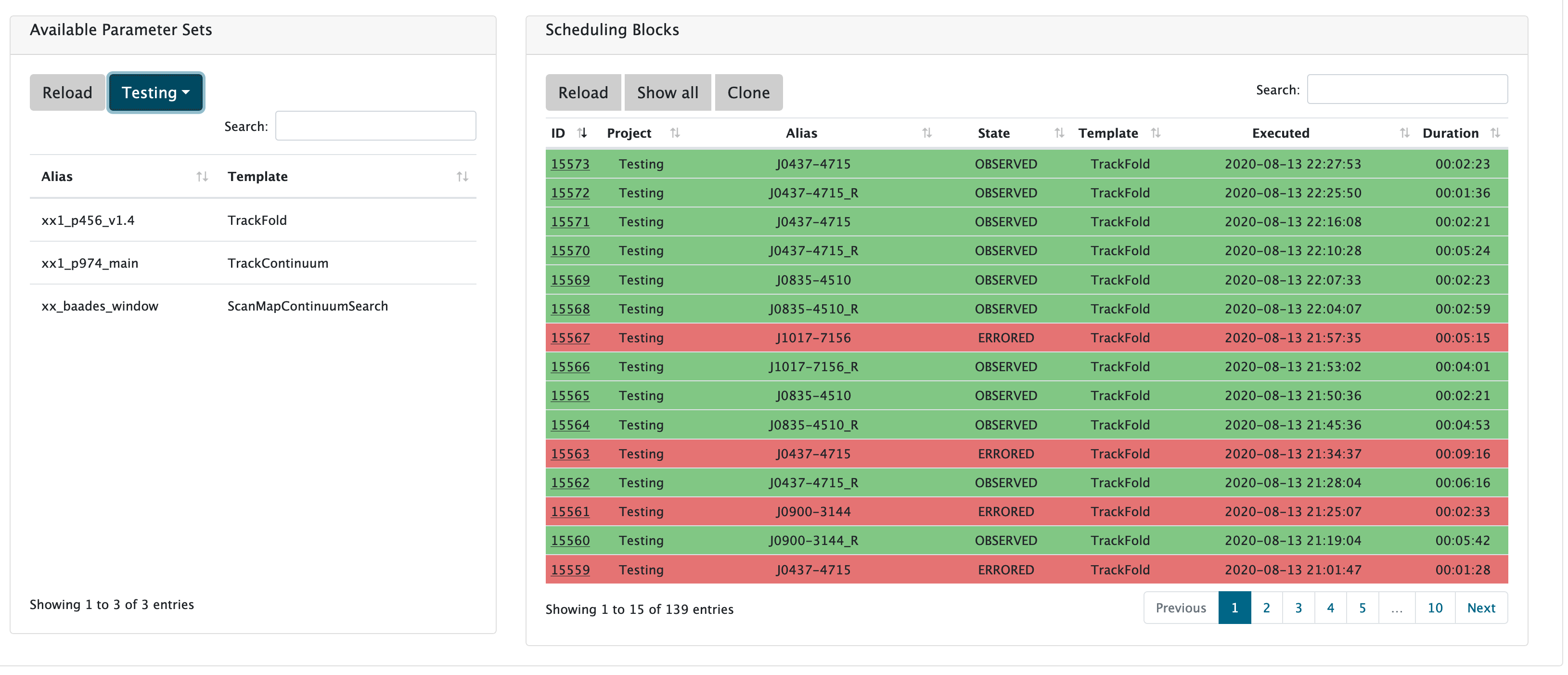
The colours of Scheduling Blocks map to their state:
- DRAFT: Orange
- SUBMITTED: Yellow
- SCHEDULED: Blue
- OBSERVED: Green
- ERRORED: Red
For each Scheduling Block, there is a link associated with the ID. Clicking on this link brings up the Scheduling Block Management Tool.
These are Annotations associated with the Scheduling Block. In the example below, the details associated with the creation of the Scheduling Block are shown.
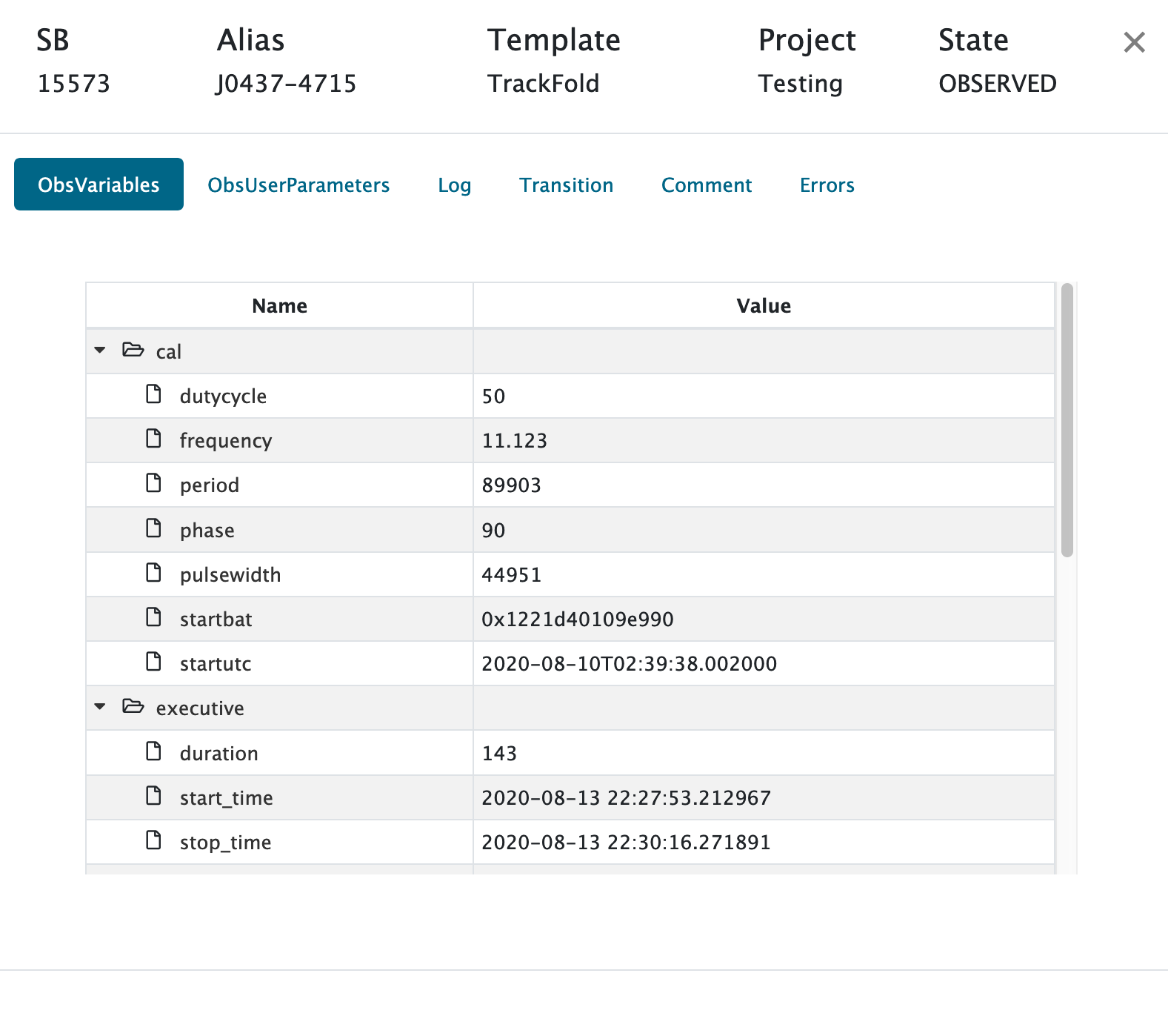
This represents the parameter set of the Scheduling Block. It is not possible to edit the parameter set from here.
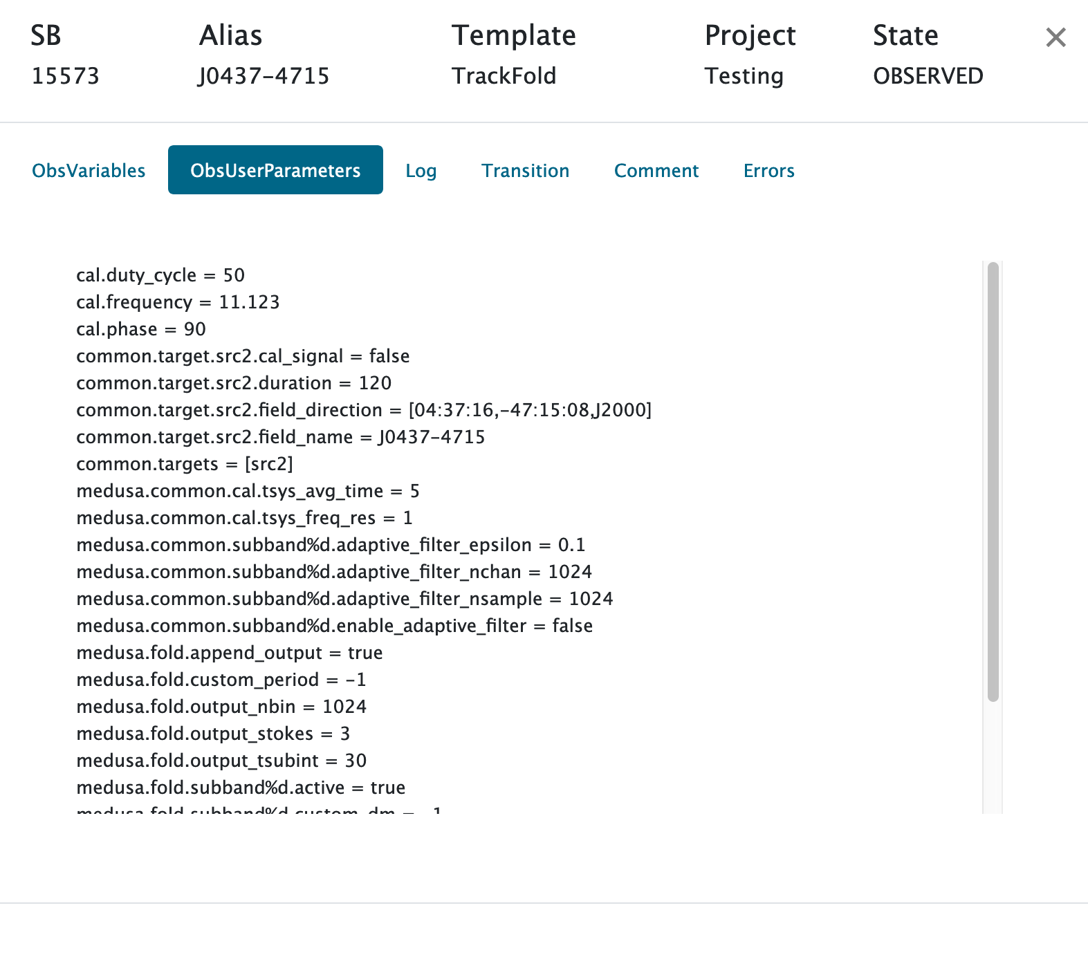
The Log tab presents the observer with execution logs. If there are errors associated with a Scheduling Block, here is where to look (and put in a Jira ticket?)
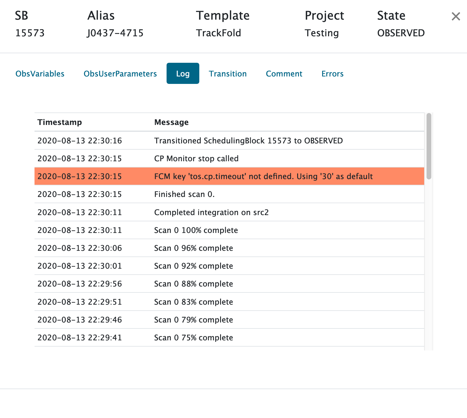
The State Transition tab allows the observer to transition a Scheduling Block. This may be useful, for example if the Scheduling Block was currently in the ERRORED state because of an incorrect parameter set, you can transition to RETIRED. Another example is when a Scheduling Block is in the ERRORED state, but the error was caused by the antenna reaching the horizon limit. If the data are good, you can transition the Scheduling Block to OBSERVED. The New state select widget will display allowed transition states for the current Scheduling Block (see here). Note a comment on the reason behind the transitioning is required.
It is possible to add comments and create Jira tickets for a Scheduling Block by clicking on the Comment button. A text entry field appears and comments can be entered and saved. This is useful for projects to keep a central record of any observing, processing or general comments relating to the Scheduling Block. Comments are saved as an annotation. If there is an issue associated with a Scheduling Block, the observer can submit a Jira ticket. If a Jira ticket exists, a link to it will be provided. Currently a CSIRO NEXUS account is needed to login to Jira to view the ticket, but eventually comments entered directly into the Jira ticket could be shown here instead of just a link.
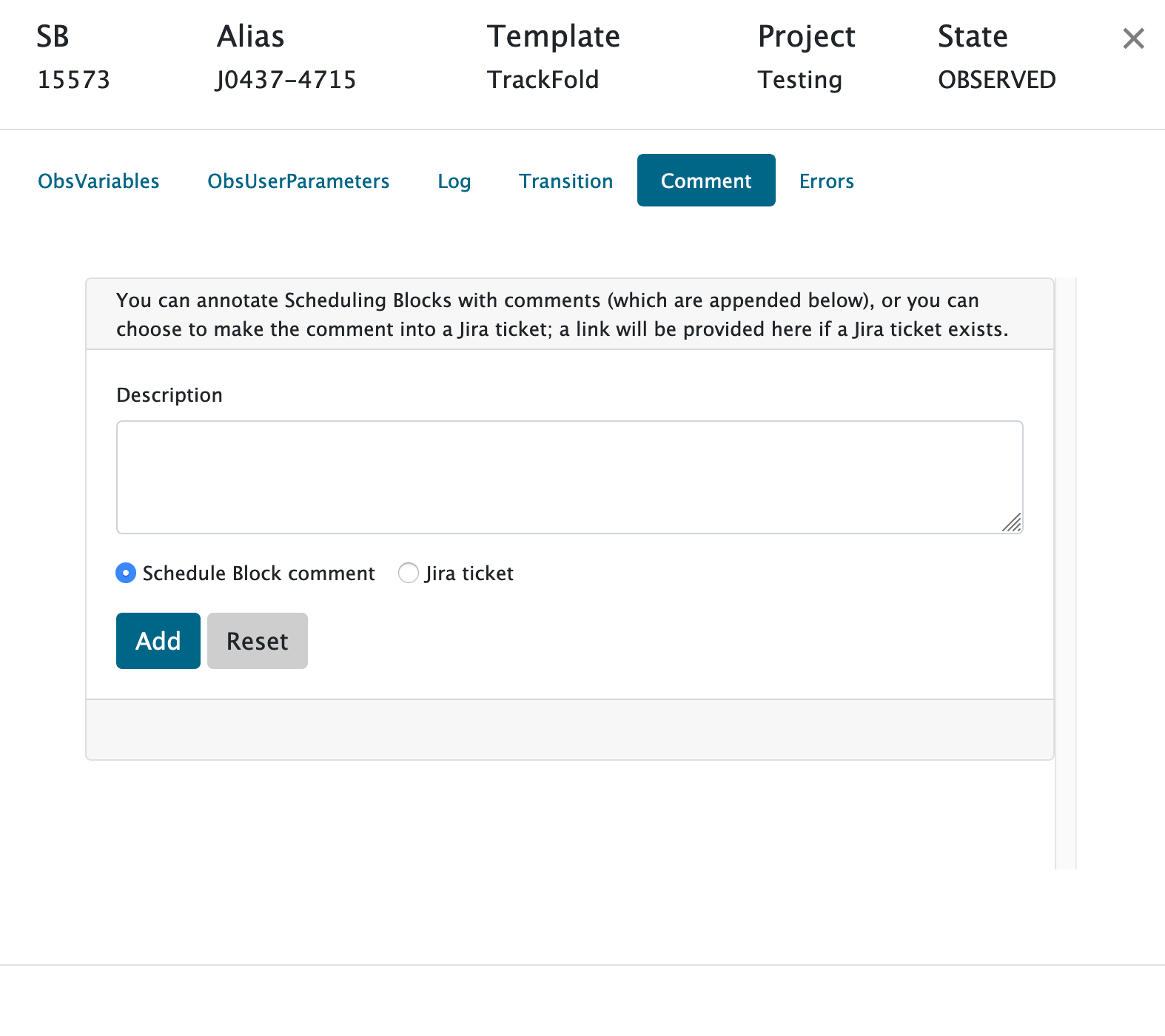
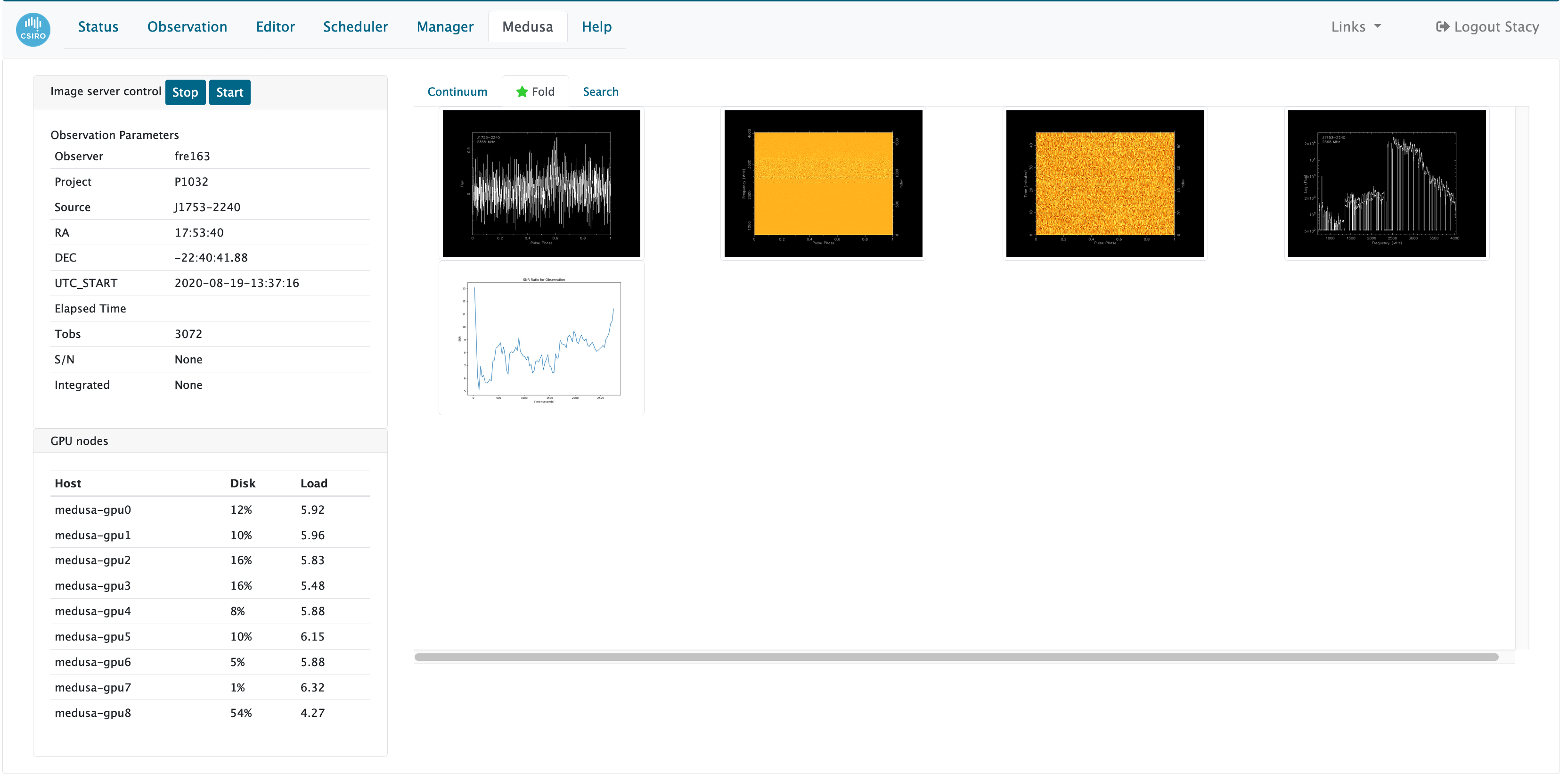
This tab provides an in-built alternative to the SPIP webpage, which requires either access from the CSIRO internal network, or SSH tunnelling (see Section 3.1.2.2). On the top left, there is an panel with options to stop and start the Dhagu? image service. If you notice plots have not been updating (they should every 10 seconds), then try restarting the service; this is not associated with , but an internal process within Dhagu? to retrieve plots and information from .
Below the image server control, is the Observational Parmameters panel. This contains information about the source currently being observed. The next panel relates to the GPU status. If you notice the disk usage is high (85%+), you may have to stop observing briefly, to allow the data to be transferred from , to the data staging server euryale.
On the right are tabs for each mode, Continuum, Fold and Search. Whichever is currenty active is identified with a green star; Fold mode is in operation for the example below. Clicking on any tab will show plots associated with that mode, but blank plots if that mode is not in operation. Note with commensal modes, at most any two tabs will be indicated as active.
The telescope is stowed for maintenance and following weather events such as strong winds. To stow the telescope, when using Dhagu?, use the STOW button under the Observation tab. If the telescope is stowed, submitting a new observation will unstow the telescope automatically. You will need to have the Observing Queue running, which is done via the START button under the "Observing" tab. You can also still use the joffrey:1 VNC session, and locate the UWL 'CS-Studio' GUI. On this window is a button to unstow/stow/park the telescope. If the UWL gui is not running, it can be restarted from the tools on the bottom bar of the VNC window. The status of the telescope when undergoing a park/stow/unstow can be seen on FROG, or the CS-Studio GUI.
When the telescope is parked, it is possible that it can drift into the ‘dead zone’. This is the Zenith angle currently defined by the range 0.95 to 1.15 degrees- the antenna park position is 1.2 degrees. If the antenna falls within this zone (check FROG), you will hear an audible alarm from FROG. In order to exit this zone, you can hope the wind will push the antenna back out, or manually stow and then unstow the antenna.
There are two main weather phenomena that could cause you to lose observing time - high winds and lightning (on rare occasions extreme heat may also affect the ability to observe with given receivers). In the case of heat stows, directions will be posted on the PORTAL.
A good source of weather information is the Weatherzone site for Murriyang.
Wind Parks: The dish has a large surface area, and under high winds it can experience forces that can render the dish unsafe for continued observing. For safety, whenever the winds pick up to levels that are considered unsafe, the control system will automatically take control and drive the dish to the Zenith (the safe position). This is referred to as a wind park. This will usually occur whenever the winds are around 40 to 45 kph. But, it does depend on other factors such as tip angle, wind direction and motor currents. For a full description of wind parks, see Section 3.6.3
Storm Stows: The Observatory has three sources of power - mains power, backup generator and UPS (batteries). Whenever there is a storm, there is often a high likelihood of lightning, too. The lightning can cause a disruption to the supply authority mains power. Normally, whenever we lose mains power, the generator should start automatically and provide power until the mains returns. If the generator fails to start however, then the drive UPS has sufficient power to allow you to drive the dish to the zenith and fully stow it. In this position the dish is guaranteed to be safe.
With the advent of remote observing, we have adopted a very conservative approach to lightning. We don’t ever want the situation arising of having the dish tipped over in a storm with high winds, and no power to stow it and make it safe. So, whenever lightning is detected, and while we still have power, the control system automatically takes control to stow the dish and make it safe. This is referred to as a Storm Stow. The dish remains stowed until the storm passes and the lightning levels drop to zero. The dish is then released and normal observing resumed.
FROG will produce audible alarms if a TPS monitoring point has its alarm state transition to true. The popup will inform the observer what the issue is. Depending on the severity, the TPS may take control of the antenna and stow. The observer has the ability to mute alarms, but note that if the TPS issues the alarm again, the mute will need to be redone.
An Alerta system is being developed, which will provide an audible alarm when any telescope subsystem transitions from a status of OKAY. As with FROG, a message indicating the problem (and possible solution), along with the severity of the issue will be indicated. It will be possible for the observer (and staff) to “shelve” the alarm, thereby removing it from the list. It will also be possible to click on a link, which points to a Grafana monitoring page, to allow people to drill down into the nature of the problem.
The status of the backend can be monitored in three ways:
Once you have initiated your observations, check that your parset has been successfully interpreted by . You can check this either under the `’ tab on Dhagu? or on the webpages. In the latter case, the page headers should read either “Idle” or “Recording” followed by your observation type (i.e. `Fold’, `Search’, or `Continuum’).

Note the “recording” status (it will be “idle” if is not recording) and check the UTC_START. This is the start time of the observation and the archived data files will have a name based on this date and time.
Note that a set of plots are given for each sub-band. At the start of each observing file, it is also good to confirm that the plots are updating correctly. It is possible for the observation header to update, but the plots do not. If the plots seem stalled, or are associated with previous observations, try stopping and starting the instrument.
Look carefully for mis-configured parameters:
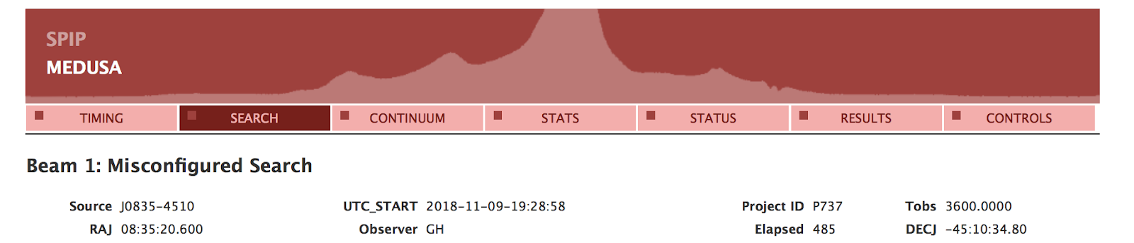
If you see `Misconfigured’ at the top of your observing page header, there is something wrong with your Parameter Set. Stop your observations, check your Parameter Set, and resubmit in order for to configure itself properly.
The status of the GPU workload can be seen on the tab of the Dhagu? webpage. If the `Disk’ and/or ‘Load’ status bars are red, consider stopping your experiment until the nodes have caught up with your observing load. If your observations will produce extremely-high data volumes (>100 GB/hour), be sure to have discussed your observing plan with and euryale experts to be sure the system can support your data rate.
The same status icons listed above can also be monitored on the webpages underneath the `Status’ tab. This page has the added bonus that you can also monitor the Shared Memory Ring Buffer statuses. Red SMRB indicate that you may be dropping packets and have incomplete data.
On the Controls Page, which can be accessed by selecting the `Controls’ tab from any webpage, it is possible to monitor any issues within the server controls of each of the GPUs. There are also global buttons near the top of the page that allow you to stop or start the backend.
If the circles on the control page are gray, or you believe that the system has stopped working (plots are not updating etc.) then click on “Stop Instrument” at the top of the webpage. Wait at least 60 seconds. All the lights should now be red. Then click “Start instrument” and again wait at least 60 seconds. If that fails then contact local staff.
When starting , all the Individual Server Controls must be OFF (red or grey). Click the Start Instrument button once and wait for the all the controls to change from OFF (red/grey) to ON (green).
When stopping , all the Individual Server Controls must be on (green). Click the Stop Instrument button once and wait for all the controls to change from ON (green) to OFF (red/grey).
Killing , should only be used if the Stop function fails to shutdown within the allotted 120s timeout. Click the Kill Instrument button once and wait at least 30 seconds for the controls to change to OFF (red/grey). When they are all red/grey you may click Start Instrument.
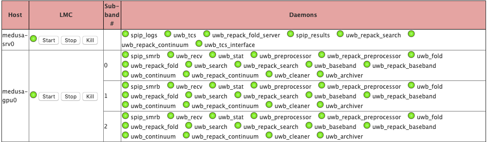
The SERVO computer monitors the speed and direction of the wind from the (default) paddock sensor, and will stow the dish automatically above limits (defined in the table below) to ensure the safety of the antenna. Winds can be monitored with FROG, the MoniCA displays in the joffrey:1 VNC.
Table 3.1. Wind Stow Limits
| Anemometer | Peak (km/h) | Gust (km/h) | Average (km/h) |
|---|---|---|---|
| Ane #1 (Az front) | 58 | 54 | 42 |
| Ane #1 (Az back) | 46 | 42 | 35 |
| Ane #2 (Az front) | 66 | 62 | 48 |
| Ane #2 (Az back) | 53 | 48 | 40 |
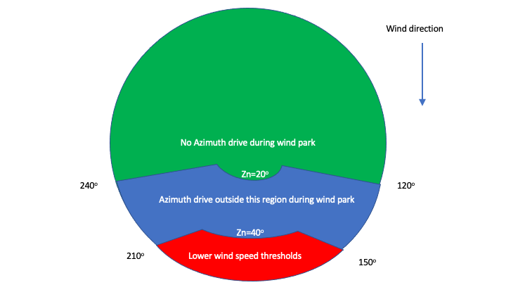
A decision to wind stow will always result in a drive to 1.2 degrees in Zenith, and in some cases will also involve a drive in Azimuth. The final Azimuth will depend upon both the starting position relative to the wind (in Azimuth and Zenith), and the proximity of the Azimuth limits. If the starting position of the dish relative to the wind is in either of the blue or red regions above (Zn > 20 deg. and 240 > Rel.Az > 120 degrees) it will be driven to the nearest relative Azimuth beyond 120 or 240 degrees; except that if such a drive would encounter a telescope limit, the longer drive will be chosen. A starting position anywhere in the green region will only produce a drive in zenith.
The wind speed thresholds that trigger a wind stow are reduced when the telescope is tilted beyond 40 degrees of Zenith and the wind Azimuth is within 30 degrees of the back of the dish (Zn > 40 deg. and 210 > Rel.Az > 150 deg.) which is the red region on the above diagram. SERVO receives data from both site anemometers continuously, and reads once per second. Since the anemometers only produce a new speed measurement every four seconds, SERVO should see four consecutive identical readings. A PEAK wind event is defined as a single anemometer measurement above the peak threshold — in order to allow for data transmission errors, SERVO checks two consecutive readings before declaring a PEAK event. A GUST event is less severe and is defined as more than one anemometer measurement above the relevant threshold in 3 minutes — SERVO checks for five readings in a hundred and eighty. An AVERAGE wind speed trigger requires that 75% of measurements are above the threshold — SERVO commences a wind stow when it sees 15 such readings in 20 seconds.
SERVO also monitors Zenith drive currents. It triggers a low current stow if the Zenith drive is enabled and not slewing upwards but the aggregate current in the two motors falls below 0.5 Amps for more than 3 seconds in 2 minutes. It triggers a high current stow if the current in either motor exceeds 30 Amps for more than 6 seconds in 1 minute.
Caution
If the wind is particularly high, the antenna can be driven into the Zenith hardware limit past 1.2 degrees. You will need to exit the limit by using the STOW button in Dhagu?, and then submit a Scheduling Block to unstow the antenna when conditions ease. You can still use the CS-Studio GUI in the joffrey:1 VNC by using stow/unstow buttons on the CS-Studio GUI (Figure 3.6).
Caution
Once an automatic wind park has occurred, the antenna must not be moved until permissible conditions have prevailed for at least 10 minutes before restarting the Observing Queue. If conditions are poor, the antenna must be fully stowed.
The telescope Protection System will automatically stow the telescope in the event of significant lightning strikes. There are three radii: Far (20-56km); Near (10-19km); and overhead (less than 10km). The numbers of strikes are weighted with those ‘far’, ‘near’ and ‘overhead’ respectively as x1, x10 and x45. The number of weighted strikes are summed and if the total is: 22 - 52, a storm warning is given; 52 - 102, a suggestion is made to start generators; 102 - 202, generators are started automatically; > 202, telescope is stowed automatically. The stow is released (and generators turned off) once levels drop below the thresholds.
We realise that observers are busy people who cannot always be in front of their observing computer for the entire duration of their experiment. The observatory can be operated in “unattended” mode when it is convenient to do so. This section describes how best to observe in this way, and what is expected from you during your experiment.
When we talk about “unattended observing”, we mean any period during your experiment where you are not immediately aware of the state of the telescope. You may be any distance away from your observing computer, or asleep, or otherwise engaged in another activity, but you are listed as the “observer in charge” on the PORTAL and can be reached in an emergency through your designated contact number.
The observatory does not require you to be responsible for the safety of the telescope equipment or of personnel. We have sophisticated systems and procedures which should handle any unsafe situation that might arise during a normal observation. For example, the automated systems (TPS described in the preceding section) will turn on the generators when a storm is approaching, and turn them off when it passes. It will also automatically handle stowing in periods of high wind, or when there is a high chance of lightning strike.
We do however expect that you are solely responsible for monitoring the quality of your data, and we do expect to be able to contact you via the phone number you supplied when you registered as the observer in charge. You should consider how often you need to check your data quality, given how much time you could lose if something goes wrong.
Telescope safety resides with the National Facility and is intended to be automated. However this does not preclude the potential for unforeseen events.
To request Remote Observer Training, email atnf-parkes-remobs[at]csiro.au
Issues related to data archiving or data access, email Lawrence Toomey: Lawrence.Toomey[at]csiro.au
The Emergency Contact Person (ECP), phone: +61 427 001 583
The Observer-in-Charge (OiC) re-direct phone number: +61 2 6861 1750
The Observing Expert: All projects will have a nominated project expert. This is a person assigned by the PI of the project to be the “go to” person for members of the team whenever a problem arises during an observation. It should be someone who is sufficiently knowledgeable and experienced to troubleshoot any problems that may arise.
To submit a fault report, email parkes.support[at]csiro.au with as much detail on the nature of the problem as possible.
High time resolution data sets are available from CSIRO’s data archive (the Data Access Portal, DAP, https://data.csiro.au) and high frequency resolution data from the Australia Telescope Online Archive (ATOA, https://atoa.atnf.csiro.au).
The standard procedure is that the raw data sets from all observations are publically available after an 18 month embargo period (from the date of the observation), or in the case of a Target of Opportunity, within a week. Any deviation from this procedure, for example a longer embargo period, has to be through agreement with the CASS Director and with approval from the ATNF Steering Committee (or through contracted telescope time).
Data is archived as soon as possible following observations. This archiving process is contingent on projects adhering to the data rates that they proposed in their OPAL proposals. If the data rate is exceeded in the observations (with the use of additional unrequested modes or capabilities) the data archiving may be interupted, and in extreme circumstances may need to be deleted to allow other scheduled projects to proceed.
High time resolution data sets are stored in PSRFITS fold and search files. Within 2 weeks of observation they are available for access from https://data.csiro.au. Various access mechanisms are possible including:
- Web download from https://data.csiro.au using OPAL or NEXUS account for sign in
- Access from CSIRO high performance computing systems
- Searching using VO tools such as TOPCAT (http://www.star.bris.ac.uk/~mbt/topcat)
For more general DAP information and assistance:
- https://confluence.csiro.au/display/dap/Download+Data
- https://confluence.csiro.au/display/dap/Download+via+WebDAV
- Contact Research Data Support at researchdatasupport@csiro.au or phone: +61 2 4960 6086
Information on data access for CSIRO computer (and HPC) account holders can be found on:
- https://confluence.csiro.au/display/AS/Data+access+-+CSIRO+computer+account+users
For non-CSIRO users, information on data access can be found on: https://bitbucket.csiro.au/projects/CPDA/repos/pks_data_access_docs/browse
Standard meta-data are stored within each PSRFITS file (as defined in https://www.atnf.csiro.au/research/pulsar/psrfits_definition/PsrfitsDocumentation.html). Currently all o bservations with the UWL are assumed to be tracking observations of a given source. The meta-data therefore only contains the right ascension and declination of the source at the start of the observation.
Pulsar fold-mode observations (and related calibration files) can be processed using the PSRCHIVE (http://psrchive.sourceforge.net/) and pfits software suites.
Calibration solutions that enable both polarisation and flux calibration are available for download from https://doi.org/10.25919/5ce76bf409bcf (and described in Hobbs et al., submitted to PASA). Typical processing commands would be:
- Use pfits_zapUWL for automated RFI flagging
- Use pfits_zapProfile on the output for any final manual flagging required
- Use psrsh for calibration with a script similar to:
          load <filename>
          install par <best parameter file>
          cal load hybrid <alfile> <pcm calibration file>
          cal
          cal frontend
          cal load <flux cal file>
          cal flux
Then further processing tasks (such as selecting specific bands of interest, or frequency and time averaging) can be carried out.
Pulsar search mode observations can be processed using DSPSR (http://dspsr.sourceforge.net/) to fold the data at the period of a known pulsar and to extract individual pulses. The output is then a fold-mode profile which can be processed as described above. To search for new pulsars then PRESTO (https://www.cv.nrao.edu/~sransom/presto/) or the SIXPROC (https://github.com/SixByNine/sigproc) version of SIGPROC can be used (note that default SIGPROC can not process PSRFITS search mode files).
The spectral line and continuum data sets are stored in the Australia Telescope Online Archive (ATOA; https://atoa.atnf.csiro.au). For the wide-band receiver, each observation is recorded in Single Dish Hierarchical Data Format (SDHDF). Details on the SDHDF format are available from: https://bitbucket.csiro.au/projects/CPDA/repos/sdhdf_docs/browse
Web download is the only access method for the SDHDF data files. Meta-data stored within each SDHDF file is obtained from two sources: (1) the starting positions and parameters for the observation and (2) information that gets updated throughout the observation (such as the current telescope position for scanning observations).
The SDHDF data sets can be loaded using standard HDF5 reading tools (that exist within packages like Python). However, we do not yet have a well-tested suite of software for processing these data. We have test versions (currently available from local staff) of software to:
Visualise spectra: in C and in python (https://bitbucket.csiro.au/projects/CPDA/repos/sdhdf_tools/browse) Convert the HDF5 format files to SDFITS. Apply a basic flux, bandpass and polarisation calibration assuming that the switched calibration signal was run throughout the observations.
All papers that make use of the Murriyang, or the online archives requires the inclusion of the acknowledgements listed here..
Observations with the UWL should reference Hobbs et al. 2020 for the receiver and observations with the 20cm Multibeam receiver should reference Staveley-Smith et al. 1996.
A
- Acknowledgements, Publishing results
- Antenna modes, Observing Strategies
C
- Constraints
- changing receivers, Changing receivers
- dead-zone, Zenith Dead Zone
- heat stow, high winds, lightning, Weather
- storm stow, Weather
- wind park, Weather
- Zenith, Scanning, Avoiding Zenith
D
- Data
- ATOA, High frequency resolution data sets (Spectral line)
- data access, Access your data and data analysis
- pulsar data, High time resolution data sets (Pulsar)
- spectral-line data, High frequency resolution data sets (Spectral line)
- Documentation
- conventions, Conventions
E
- Emergency Contact Person
- contact, Key contact numbers
- when to call, Observing Tab
G
- Green Time
- applying for, Directors Discretionary Time / Unallocated time / "Green time"
- booking via PORTAL, Book Tab
M
- MEDUSA
- apollocat, Pulsar Fold Mode
- Commensal modes, Commensal Observing Modes
- Continuum/Spectral-line mode, Spectral-line / Continuum Modes
- Fold mode, Pulsar Fold Mode
- frequency range, Ultra Wide-bandwidth Low (UWL)
- introducing, MEDUSA
- Search mode, Pulsar Search and Single Pulsar Modes
- Voltage capture, Voltage Capture Modes
- Zooms, Zoom Modes
O
- Observer-in-Charge
- contact, Key contact numbers
- Observing Expert
- Observing Tools
P
- Parameter Set, Viewing and Saving the Parameter Set
- continuum/spectral-line mode, Example CONTINUUM (Spectral-line) Parmameter Set
- fold mode, Example Pulsar FOLD Parameter Set
- fold mode; MARS receiver, Example FOLD Parameter Set: J0835-4510 with MARS
- scan mode, Example SCAN Parmameter Set
- scanmap continuum/spectral-line mode, Example SCANMAP CONTINUUM (Spectral-line) Parmameter Set
- search mode, Example Pulsar SEARCH Parameter Set
R
- Receivers, Receiver Fleet
- K-BAND, 13MM, K-Band (13MM)
- MARS, MARS
- Methanol, Methanol (‘Old Meth’)
- UWL, Ultra Wide-bandwidth Low (UWL)
- Remote Observing, Observer Training
- Observer-in-Charge, Observing Tab
- passwords, Observer Training
- RFI, Interference & Avoiding RFI
- "mid-week", Interference & Avoiding RFI
- RFI weathermap, RFI Weathermap
- satellites, Satellite RFI
S
- Signal-Path, Signal Paths
- MEDUSA, Signal Paths
- PCS, Signal Paths
- SSH access, Login to VNCs from outside CSIRO/ATNF
T
- Telescope Protection System
- alarms, Audible alarms
- in Dhagu?, Health
- in FROG, Status
- introducing, Telescope Protection System
U
- UWL
- frequency range, Ultra Wide-bandwidth Low (UWL)
- introducing, Ultra Wide-bandwidth Low (UWL)
W
- Web browser support
- Firefox, MS Edge, Google Chrome, Web browser support
- Wind
- back of the dish, FROG (Fantasic Remote Operations GUI)
- in FROG, FROG (Fantasic Remote Operations GUI)
- limits, FROG (Fantasic Remote Operations GUI)
- stow, limits, Wind Stows
- trend, FROG (Fantasic Remote Operations GUI)
- Wrap limits, Tracking, FROG (Fantasic Remote Operations GUI)